Last time, we introduced the action and the Lagrangian. This time, we'll do some examples to try to demystify it!
Solving for the motion of a physical system with the Lagrangian approach is a simple process that we can break into steps:
- Set up coordinates.
- Write down the total kinetic energy \( T \) and potential energy \( U \).
- Apply the Euler-Lagrange equation to each coordinate \( y_i \),
\[ \begin{aligned} \frac{\partial \mathcal{L}}{\partial y_i} - \frac{d}{dt} \left( \frac{\partial \mathcal{L}}{\partial \dot{y_i}} \right) = 0. \end{aligned} \]
- Solve the resulting equations of motion for given initial conditions.
Example: free fall
Consider a particle of mass \( m \) in free-fall, moving in the \( y \)-direction. We only need one coordinate, which is \( y \), the height of the particle. The gravitational potential is just \( U = mgy \), so our complete Lagrangian is
\[ \begin{aligned} \mathcal{L} = T - U = \frac{1}{2} m \dot{y}^2 - mgy. \end{aligned} \]
The derivatives of the Lagrangian we need are
\[ \begin{aligned} \frac{\partial \mathcal{L}}{\partial \dot{y}} = \frac{\partial T}{\partial \dot{y}} = m \dot{y} \\ \frac{\partial \mathcal{L}}{\partial y} = \frac{\partial U}{\partial y} = mg\\ \end{aligned} \]
so the Euler-Lagrange equation is
\[ \begin{aligned} \frac{\partial \mathcal{L}}{\partial y} = \frac{d}{dt} \left( \frac{\partial \mathcal{L}}{\partial \dot{y}} \right) \\ -mg = m \ddot{y} \end{aligned} \]
So extremizing the action gives us the usual equation, \( \ddot{y} = -g \). Notice that if we instead try to extremize the total energy \( E = T + U \), the sign flips, \( \ddot{y} = g \) - we predict that the particle falls up! In some sense, the Lagrangian captures the fact that there is a tradeoff between kinetic and potential energy in mechanical systems.
Of course, you could complain that "moving in the \( y \)-direction" is a strong assumption to make. What if I want to look at the trajectory of a projectile in the \( x-y \) plane? I can go back and add the missing \( x \) coordinate to the Lagrangian:
\[ \begin{aligned} \mathcal{L} = \frac{1}{2} m (\dot{x}^2 + \dot{y}^2) - mgy. \end{aligned} \]
We pick up an additional Euler-Lagrange equation for \( x \), but since \( x \) doesn't appear in the potential, it's a trivial equation:
\[ \begin{aligned} \frac{\partial \mathcal{L}}{\partial x} = \frac{d}{dt} \left( \frac{\partial \mathcal{L}}{\partial \dot{x}} \right) \\ 0 = m \ddot{x} \end{aligned} \]
If there is a coordinate in our problem which doesn't show up in the potential at all, we say that it is ignorable - there is no interesting dynamics in that direction, and if we set \( x(0) = \dot{x}(0) = 0 \) then there's no motion in \( x \) at all.
Example: mass on a spring
Suppose we have a mass \( m \) on a spring with spring constant \( k \), and the spring is unstretched at \( x=0 \).
The kinetic energy is just \( \frac{1}{2} m \dot{x}^2 \), the same as in our free-fall example.
Clicker question
What is the Lagrangian of the mass and spring system?
A. \( \mathcal{L} = \frac{1}{2}m\dot{x}^2 + \frac{1}{2}kx^2 \)
B. \( \mathcal{L} = \frac{1}{2}m\dot{x}^2 - \frac{1}{2}kx^2 \)
C. \( \mathcal{L} = \frac{1}{2}m\dot{x}^2 + kx \)
D. \( \mathcal{L} = \frac{1}{2}m\dot{x}^2 - kx \)
Answer: B
The potential energy of a mass on a spring is \( U = +\frac{1}{2} kx^2 \), and we should be careful about the sign! The spring potential \( U \) has a plus sign, because if we increase (or decrease) \( x \), the spring is stretched (or compressed) and it should have more potential energy. Alternatively, you may have remembered that the spring force is restoring, so \( F = -kx \); remembering that \( F = -\nabla U = -dU/dx \) also matches our positive potential \( U \) above. Using \( \mathcal{L} = T - U \) then gives us choice B.
As with the first example, we have to make sure we get our signs correct!
The derivatives of the Lagrangian are
\[ \begin{aligned} \frac{\partial \mathcal{L}}{\partial x} = -kx \\ \frac{\partial \mathcal{L}}{\partial \dot{x}} = m\dot{x} \end{aligned} \]
so the Euler-Lagrange equation is
\[ \begin{aligned} \frac{\partial \mathcal{L}}{\partial x} - \frac{d}{dt} \left(\frac{\partial \mathcal{L}}{\partial \dot{x}}\right) = 0 \\ -kx - m \ddot{x} = 0 \\ \ddot{x} = -\frac{k}{m} x. \end{aligned} \]
which should look very familiar to you! We won't proceed any further, but you'll recall that this is a simple oscillator - solutions to this differential equation are sines and cosines, since applying two derivatives to those functions gives you back the same function with a sign flip.
In these very simple examples, it's hard to appreciate the power of the Lagrangian reformulation of classical mechanics. Writing down the Lagrangian and the resulting Euler-Lagrange equations for something like a mass on a spring must seem like an unnecessary complication. The main advantage of the Lagrangian is that it is a problem involving only energy - only scalar quantities - while to apply Newton's laws, you have to think in terms of vectors.
Let's do one more example that will show off a little more of the power of Lagrangian mechanics.
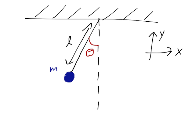
Example: the simple pendulum
Let's do an example using the Lagrangian approach to see how simple things can be when we move away from Cartesian coordinates, and which will showcase some other interesting properties. Consider a simple pendulum of length \( \ell \) and bob mass \( m \):
Starting in Cartesian coordinates, we know how to write down the kinetic and potential energies:
\[ \begin{aligned} \mathcal{L} = T - U = \frac{1}{2}m\dot{x}^2 + \frac{1}{2} m\dot{y}^2 - mgy. \end{aligned} \]
This is the same Lagrangian as a particle in free-fall; what we're missing is the fact that this is a pendulum, and the bob is attached to a rod. This gives a constraint on the motion - at any instant, the particle has to be distance \( \ell \) from where the rod is attached,
\[ \begin{aligned} x^2 + y^2 = \ell^2. \end{aligned} \]
This constraint lets us eliminate one of the two variables; if we specify either \( x \) or \( y \), we know immediately the other coordinate. Of course, \( x \) and \( y \) aren't the only quantities we can use to describe the pendulum; we know that we usually prefer to work with the angle \( \theta \) that the pendulum makes with the vertical. So let's change coordinates like this:
\[ \begin{aligned} x = \ell \sin \theta \\ y = \ell (1 - \cos \theta) \end{aligned} \]
so the derivatives are
\[ \begin{aligned} \dot{x} = \ell \dot{\theta} \cos \theta \\ \dot{y} = \ell \dot{\theta} \sin \theta \end{aligned} \]
and the Lagrangian becomes:
\[ \begin{aligned} \mathcal{L} = \frac{1}{2} m \ell^2 \dot{\theta}^2 - mg\ell (1 - \cos \theta). \end{aligned} \]
Notice that the kinetic energy looks very familiar: it's exactly the rotational kinetic energy of the bob, \( \frac{1}{2} I \omega^2 \), or \( \frac{1}{2} mv^2 \) with \( v \) pointing in the tangential \( \hat{\theta} \) direction.
Now here's the fun part. I'm just going to forget that I changed coordinates, and try to write down the Euler-Lagrange equation for the variable \( \theta \). What I find is:
\[ \begin{aligned} \frac{\partial L}{\partial \theta} = -mg\ell \sin \theta \\ \frac{\partial L}{\partial \dot{\theta}} = m \ell^2 \dot{\theta} \\ \frac{\partial L}{\partial \theta} - \frac{d}{dt} \left(\frac{\partial L}{\partial \dot{\theta}}\right) = 0 = -mg\ell \sin \theta - m\ell^2 \ddot{\theta} \end{aligned} \]
or dividing through,
\[ \begin{aligned} \ddot{\theta} + \frac{g}{\ell} \sin \theta = 0. \end{aligned} \]
This is the correct equation of motion for a pendulum derived using Newton's laws! We didn't have to treat \( \theta \) any differently just because it was an angle; all we had to do was carry out a single change of coordinates. Fundamentally, this works because Hamilton's principle and the Euler-Lagrange equations don't care what our variables are, just that we can write the action in the standard form. In other words, we've changed coordinates but not changed the action:
\[ \begin{aligned} S = \int_{t_i}^{t_f} dt\ \mathcal{L}(t, x, \dot{x}, y, \dot{y}) = \int_{t_i}^{t_f} dt\ \mathcal{L}(t, \theta, \dot{\theta}). \end{aligned} \]
The variable \( \theta \) here is an example of a generalized coordinate (or "GC"), which in general we will denote with the symbol \( q_i \). Generalized coordinates don't have to have units of length, or even the same units as each other. They just have to be some function of the original Cartesian coordinates and time. If we have \( N \) particles in our system, we can write
\[ \begin{aligned} q_i = q_i(\vec{r}_1, \vec{r}_2, \vec{r}_3, ..., \vec{r}_N, t). \end{aligned} \]
It's important that the set of GCs that we choose allow us to uniquely specify the configuration of our physical system. In other words, the equations above have to be invertible so that we can also write
\[ \begin{aligned} \vec{r}_i = \vec{r}_i(q_1, q_2, q_3, ..., q_{dN}, t) \end{aligned} \]
Here little \( d \) stands for dimension; by default \( d=3 \) of course, but we'll commonly deal with problems (like the pendulum) where we study a two-dimensional system that's easy to draw on the board. (In the pendulum example above, the \( z \) coordinate is ignorable, remember.)
Now we're starting to see some of the advantages of the Lagrangian approach emerge. The real power of the Lagrangian comes from the fact that it only deals in scalars. To see why this is a big deal, think about what happens when we change from one coordinate system to another:
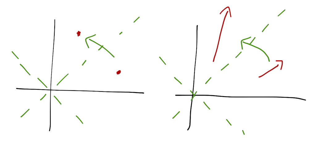
A scalar quantity is just like a point; its position as measured in the new coordinates moves, but that's it. All we need to know is the functional relationship between the new coordinates and the old:
\[ \begin{aligned} f(x',y',z') = f(x(x',y',z'),y(x',y',z'),z(x',y',z')). \end{aligned} \]
On the other hand, vectors have a length and a direction, both of which can change as we shift coordinate systems. We need not just the functional relationship between the coordinates, but also how the unit vectors themselves are changed. If we want to evaluate a gradient or a curl, we have to memorize complicated formulas which take this stretching and twisting of the vectors into account properly.
If we have multiple particles in our system, the simplicity of the Lagrangian approach is compounded further. Suppose we have three electric charges moving around in three dimensions; there are two force vectors on each particle, for a total of 18 independent components of the force to keep track of. But there is only one Lagrangian for the entire system!
Counting degrees of freedom
How many generalized coordinates do we actually need? This quantity actually has a special name: the number of degrees of freedom of a physical system is the number of GCs required to uniquely describe it. For particles moving freely in space, we see that there are \( 3N \) degrees of freedom; each particle has a triplet of coordinates \( (x,y,z) \) that we need to specify. But as we saw last time, very often we're interested in constrained systems. Our concrete example was the simple pendulum in the \( x-y \) plane:
The bob can move in 2 directions, but the presence of the string provides the constraint
\[ \begin{aligned} x^2 + y^2 = \ell^2, \end{aligned} \]
which means that we can eliminate one variable; the single generalized coordinate \( \theta \) is enough to give us both \( x \) and \( y \) for the bob. In general, counting degrees of freedom is easy:
Degrees of freedom
For a system of \( N \) particles in \( d \) dimensions, subject to \( m \) constraints, the number of degrees of freedom is
\[ \begin{aligned} n_{\rm dof} = dN - m, \end{aligned} \]
and \( n_{\rm dof} \) generalized coordinates are needed to describe the system.
Let's run through a few examples! The single pendulum above has \( d=2 \), \( N=1 \), and \( m=1 \), so we find only one degree of freedom - consistent with the one coordinate (\( \theta \)) needed to describe the system. The double pendulum is slightly more involved:
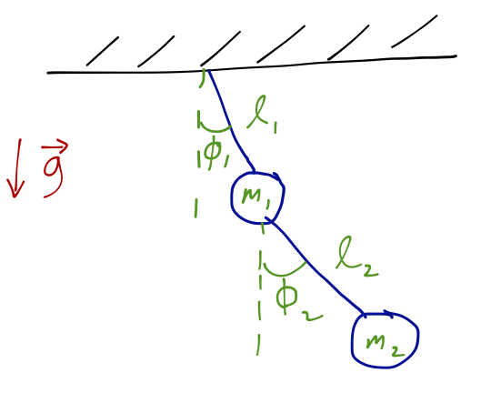
Now clearly \( N=2 \), and we identify two constraints (two strings) - so \( n_{\rm dof} = 4-2 = 2 \) (hence, two angles will work as a complete set of GCs.) This is easy to extrapolate; the \( n \)-tuple pendulum has \( n \) degrees of freedom, which are the \( n \) angles that each bob makes with the one above it.
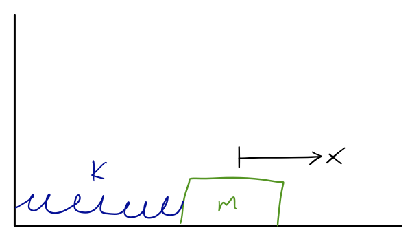
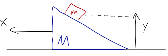
How about something a little different? Consider a block on a frictionless ramp, which is itself free to slide on a frictionless surface:
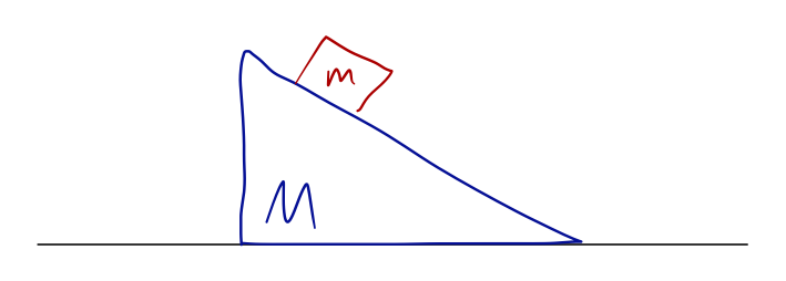
Again \( N=2 \) and \( d=2 \). We also have 2 constraints again; the block stays on the ramp, and the ramp stays on the surface. So we expect to need two coordinates. One possibility is the \( x \)-position of the ramp, and the height of the block:
But an equally valid choice for the second coordinate would be the distance the block has traveled down the ramp:
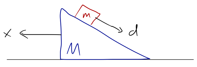
This second choice of coordinates probably looks a bit weird to you, and it's a good example of two key facts about generalized coordinates. First, in general the choice of GCs is not unique for any given problem! Of course, many problems will be significantly easier to solve with the right choice of coordinates; it will take some practice and intuition to be able to make such a choice consistently.
Second, this illustrates the key difference between generalized coordinates and the more ordinary coordinate systems that you're familiar with, e.g. spherical or cylindrical coordinates. All of the standard coordinate systems you know are orthogonal coordinate systems - which means that the unit vectors are perpendicular to one another. Here, \( x \) and \( d \) are (clearly) not orthogonal!
Doing anything with vectors in a basis which isn't orthogonal is, as you can imagine, a horrible experience. But again, now that we're using the Lagrangian approach we don't care about vectors, which means we don't care about orthogonality (or even about unit vectors.)
There is one important caveat, which is that only certain types of constraints are allowed in the Lagrangian formalism as we're using it (without violating assumptions we've made or leading to a bad change of coordinates.) Specifically, we can apply any constraint that can be written in the form
\[ \begin{aligned} f_\alpha(\vec{r}_1, \vec{r}_2, ..., \vec{r}_N, t) = 0. \end{aligned} \]
This is called a holonomic constraint. This is a somewhat formal way of writing it out: the key features of a holonomic constraint are
- It's an equation, not an inequality;
- It depends only on positions and time, not on velocities;
- It doesn't depend on any information other than the coordinates of the objects (and time.)
A physical system with only holonomic constraints is said to be holonomic; we can only apply our Lagrangian formalism to holonomic systems.
Next time: mostly more examples!