Last time, we ended with a discussion of generalized coordinates. Since the Lagrangian approach only depends on scalar quantities (energy), we don't have to worry about using only orthonormal coordinate systems; we can use any function of our original Cartesian coordinates to solve for the motion.
The number of coordinates that we need to completely describe a given system is equal to the number of degrees of freedom,
\[ \begin{aligned} n_{\rm dof} = dN - m, \end{aligned} \]
for \( N \) particles in \( d \) dimensions subject to \( m \) constraints. For our Lagrangian approach to be valid as written, these constraints must all be holonomic. A holonomic constraint satisfies three conditions:
- It's an equation, not an inequality;
- It depends only on positions and time, not on velocities;
- It doesn't depend on any variable other than the coordinates of the objects (and time.)
Clicker question
Which of the following systems are holonomic?
A. The double pendulum, but with the lower mass attached by a spring instead of a string.
B. The motion of a hockey puck around a frictionless air hockey table (with no holes in it.)
C. A bead moving frictionlessly on a circular wire hoop, which is spinning at constant angular speed \( \omega \).
D. A and B
E. A and C
Answer: E
The double pendulum is holonomic, although it's a bit counter-intuitive; there is one holonomic constraint, which is the string connecting the first bob to the ceiling. The spring connecting the second bob does not give a constraint - it just gives a contribution to the potential energy instead!
The bead on a rotating hoop is also holonomic; the wire constraint can be written as a function of space and time, but including time is okay. The angular speed \( \omega \) doesn't violate the third condition because it's a constant.
The hockey puck, however, is not holonomic; the constraints come from the boundary of the table, but that can only be written as an inequality, not an equality.
(Note: since technically the ceiling I drew on my slide for A could give a non-holonomic inequality constraint, I counted either C or E as correct answers to the clicker poll.)
As I said, we'll encounter mainly holonomic constraints in the problems we solve. The best way to recognize a holonomic constraint is actually just to recognize cases that aren't holonomic. The two most common non-holonomic constraints to watch out for are inequalities, or systems where the final state depends not just on the coordinates but on the path taken.
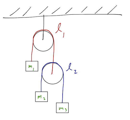
Example: double Atwood's machine
Also known as the "double pulley" system; the setup is as drawn below. The constraints are clearly holonomic, given by the strings over the (massless) pulleys. We assume, as is usual for a pulley problem, that the blocks only move up and down, and don't swing from side to side.
Clicker Question
_Which is a valid, complete choice of generalized coordinates (with no more than needed by the degrees of freedom?) _
A.
B.
C.
D.
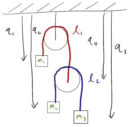
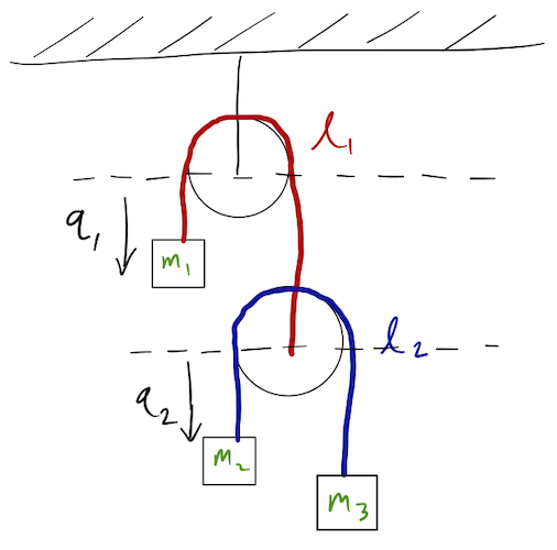
Answer: A
We can eliminate C and D just by counting degrees of freedom: we have four moving objects (the lower pulley and three blocks) in one dimension (by assumption, nothing is moving in the horizontal direction, and there are no forces that way to spoil our assumption!), so \( d=1 \) and \( N=4 \). We see two constraints: the lengths of the two ropes connecting block 1 and the lower pulley, and blocks 2 and 3. So \( n_{\rm dof} = 2 \), which means we need only 2 GCs, which means either A or B must be correct.
Note: it's equally valid to count five objects to start with, including both pulleys, and to count a third constraint, which is the rope securing the top pulley to the ceiling. I ignored that pulley completely, because it's totally fixed and doesn't take part in the dynamics.
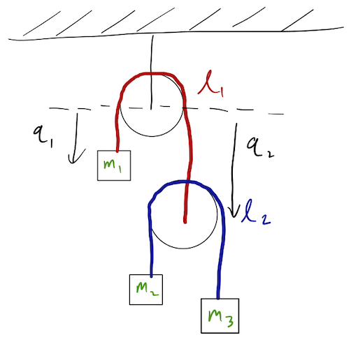
If we look at option B, we notice a problem: \( q_1 \) and \( q_2 \) as drawn aren't independent - from the rope constraint we have \( q_2 = \ell_1 - q_1 \). So really, we only have one coordinate, which isn't enough to specify the system completely. This is obvious since with just the \( q_1 \) and \( q_2 \) drawn in B, we have no way to tell where blocks 2 and 3 are relative to the lower pulley! So the only possibility is option A.
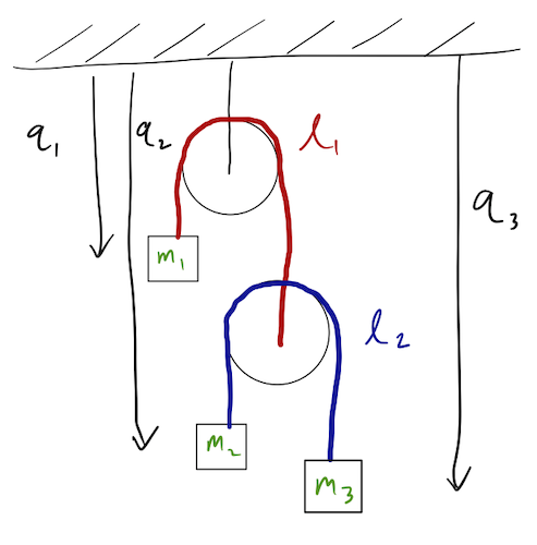
Note that if I hadn't specifically said "don't give me more coordinates than degrees of freedom", options C and D would be perfectly valid sets of GCs. However, there are constraints relating them to each other. There's nothing wrong with switching to \( q_1, q_2, q_3, q_4 \) of option D and then imposing the constraints to eliminate two of the variables. (You will, of course, end up with a description very similar to what we picked in option A.)
Let me draw out all of the positions of the blocks using the generalized coordinates we chose:
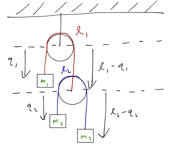
Here I am assuming the radius of the pulleys is negligible, i.e. the length of the rope which loops around the top of the pulley is much smaller than the total length \( \ell \). (Nothing interesting would change without this assumption, we'd just get an extra constant in the coordinates on the right-hand side of the diagram.)
Now, let's compute the Lagrangian. The kinetic energy is easy enough to calculate, but we have to make sure to start in the inertial frame! Let's be very careful and start with a Cartesian coordinate system: we'll take \( y \) to point up with origin at the center of the top pulley. Then the \( y \)-coordinates of the three masses are:
\[ \begin{aligned} y_1 = -q_1 \\ y_2 = -\ell_1 + q_1 - q_2 \\ y_3 = -\ell_1 - \ell_2 + q_1 + q_2 \end{aligned} \]
We always know how to write the kinetic energy in Cartesian coordinates:
\[ \begin{aligned} T = \frac{1}{2} m_1 \dot{y}_1^2 + \frac{1}{2} m_2 \dot{y}_2^2 + \frac{1}{2} m_3 \dot{y}_3^2. \end{aligned} \]
Taking time derivatives above and substituting in, we arrive back at the answer we found last time:
\[ \begin{aligned} T = \frac{1}{2} m_1 \dot{q}_1^2 + \frac{1}{2} m_2 (\dot{q}_1 - \dot{q}_2)^2 + \frac{1}{2} m_3 (\dot{q}_1 + \dot{q}_2)^2 \\ = \frac{1}{2} (m_1 + m_2 + m_3) \dot{q}_1^2 + \frac{1}{2} (m_2 + m_3) \dot{q}_2^2 + (m_3 - m_2) \dot{q}_1 \dot{q}_2. \end{aligned} \]
Very important note: this is more complicated than you might have guessed \( T \) would look! In particular, the kinetic energy of the blocks is not just
\[ \begin{aligned} T \neq \frac{1}{2} m_1 \dot{q}_1^2 + \frac{1}{2} (m_2 + m_3) \dot{q}_2^2. \end{aligned} \]
which you might guess if you went too quickly from the diagram. If you think carefully, our result for \( T \) does make sense: it's fairly obvious that the speed of, say, block \( m_2 \) will depend on both \( q_1 \) and \( q_2 \), and so we can just write down the speeds and compute everything as \( T = \frac{1}{2} mv^2 \), and we'll be fine. But the conversion isn't so obvious for every set of GCs you'll run into. When in doubt, always start in a Cartesian coordinate system and convert to generalized coordinates!
Now we're ready to move on to the potential energy. Again, it's easiest to start in our Cartesian coordinates where we know the answer:
\[ \begin{aligned} U = m_1 g y_1 + m_2 g y_2 + m_3 g y_3 \\ = -m_1 g q_1 - m_2 g(\ell_1 - q_1 + q_2) - m_3 g (\ell_1 + \ell_2 - q_1 - q_2) \\ = -(m_1 - m_2 - m_3)g q_1 - (m_2 - m_3)g q_2 \end{aligned} \]
where I've dropped all of the constant terms from \( U \), which we're of course free to do by re-zeroing the potential. (Whatever constants are there won't appear in the Euler-Lagrange equations anyway.) Combining into \( \mathcal{L} = T - U \), the Euler-Lagrange equations are:
\[ \begin{aligned} \frac{\partial \mathcal{L}}{\partial q_i} - \frac{d}{dt} \left(\frac{\partial \mathcal{L}}{\partial \dot{q_i}}\right) = 0 \end{aligned} \]
or, expanding out from above,
\[ \begin{aligned} (m_1 - m_2 - m_3) g = (m_1 + m_2 + m_3) \ddot{q_1} + (m_3 - m_2) \ddot{q_2} \\ (m_2 - m_3) g = (m_2 + m_3) \ddot{q_2} + (m_3 - m_2) \ddot{q_1}. \end{aligned} \]
This motion is, as we might expect, pretty simple; we just have two accelerations and a bunch of constants. We could go on to solve for the full motion in terms of \( q_1 \) and \( q_2 \) just by rearranging things and integrating twice, but I'll stop here - the algebra is too tedious for the blackboard. As a cross-check, we can already notice that the equilbrium points indicated by this solution make physical sense: if \( m_2 = m_3 \), then the second equation gives \( \ddot{q_2} = 0 \), which makes sense because the lower pulley is balanced. For the upper pulley, from the first equation if we have \( m_1 = m_2 + m_3 \) and \( m_2 = m_3 \), then the system is balanced and again there is no acceleration (\( \ddot{q_1} = \ddot{q_2} = 0 \).)