We've seen lots of examples now of putting the Lagrangian formalism to work to easily find equations of motion (accelerations), even for complicated physical systems. However, we haven't gone much further than that for most problems we've seen, mainly because the differential equations we've been finding are very difficult to solve!
Still, the equation of motion itself contains a lot of information, even without solving it! In particular, it allows us to identify equilibrium points where the system will remain stationary - and the presence of these points will tell us how the system moves near them, as well!
Let's go through another example to illustrate some of the interesting things we can learn from just knowing the accelerations.
Example: bead on a spinning hoop
The setup of this example follows closely from Taylor's treatment, given as Example 7.6. I usually don't like to follow the book too closely in class, since you can read it on your own, but this example is important enough that it's worth seeing twice. I'll go into a little bit more detail for the setup at the beginning.
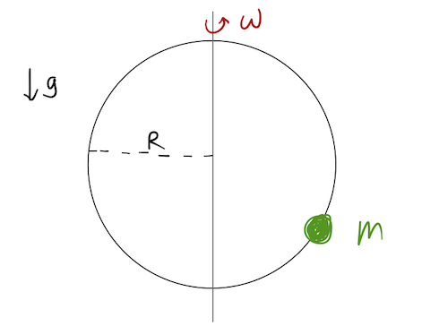
Here's the basic setup: a bead of mass \( m \) and negligible size is threaded on a (frictionless) wire hoop of radius \( R \), which is spinning at constant angular speed \( \omega \). The only force acting is gravity, pointing down in the vertical direction as usual.
As always, we should start by counting degrees of freedom!
Clicker Question
How many constraints, and how many degrees of freedom, does the motion of the bead have?
A. 2 constraints, 2 dof
B. 2 constraints, 1 dof
C. 2 constraints, 0 dof
D. 1 constraint, 2 dof
E. 1 constraint, 1 dof
Answer: B
This is, in fact, a three-dimensional problem; the bead moves in \( x \), \( y \), and \( z \) as the hoop spins around. Since we know that
\[ \begin{aligned} n_{\rm dof} = dN - m, \end{aligned} \]
with \( d=3 \) we can narrow the options down to B or D.
The question now is, how many constraints are there? Clearly, the only constraint comes from the wire, so there's just one...right? In fact, the wire provides two constraints in this problem. The first is obvious: the constraint that the bead stays on the wire. But there is a second constraint, which is the condition that the wire hoop is spinning at a constant angular rate \( \omega \). Using spherical coordinates \( (\rho, \theta, \phi) \) for the bead, we can write both constraints out as equations:
\[ \begin{aligned} \rho = R; \\ \sin (\phi - \omega t) = 0. \end{aligned} \]
(Note that trying to write this constraint as just \( \phi = \omega t \) isn't quite right, because spherical coordinates are a little awkward for the hoop: at \( t=0 \) the bead can be found at either \( \phi=0 \) or \( \phi=\pi \), notice.)
By the way, it's often a good idea to check your results against your physical intuition! Just by looking at the system, you should be able to see that there's only one way for the bead to move, whether it's spinning or not; along the wire. Since there's only one way for the bead to move, it has one degree of freedom.
Let's move on, and (as always) start in an orthogonal coordinate system before changing to our GCs. We'll define \( \theta \) to be the angle of the bead from the center of the hoop, with \( \theta=0 \) at the bottom as pictured:
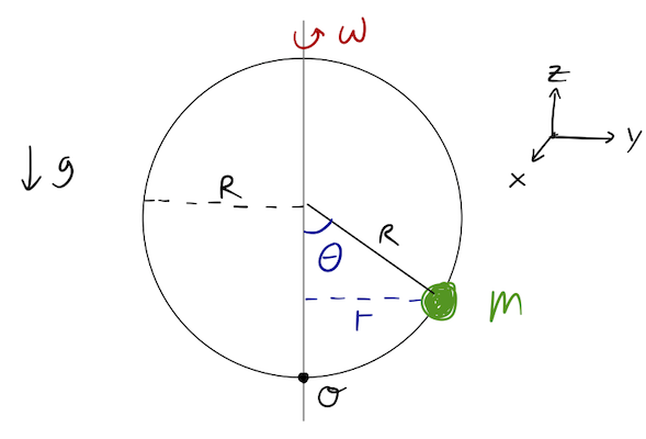
Taking \( z \) to be pointing up in the diagram and putting the origin at the bottom of the hoop as pictured, we can write
\[ \begin{aligned} z = R (1 - \cos \theta). \end{aligned} \]
Now, we could go on to write out \( x \) and \( y \) in terms of the angular speed \( \omega \) and the distance to the axis, \( r = R \sin \theta \), and then plug in to the kinetic energy in the \( x-y-z \) coordinates. However, this will be a mess of trig functions that we'll have to simplify. There must be a better way!
Aside: kinetic energy in cylindrical and spherical coordinates
In fact, any time you see angles as generalized coordinates, you should be thinking about whether you can use one of the other orthogonal coordinate systems you're familiar with: namely cylindrical (or polar in 2D) and spherical coordinates. As long as you know what the kinetic energy looks like in those coordinates, you can often find the expression you want much more quickly.
Let's go through the derivation for the kinetic energy in cylindrical coordinates, just to show you how it works (and to help you appreciate the work it will save you.)
To derive this, we'll start in Cartesian coordinates. The coordinate change is:
\[ \begin{aligned} x = r \cos \phi \\ y = r \sin \phi \\ z = z \end{aligned} \]
On notation: you'll often see \( \rho \) for the radius and \( \theta \) for the angle here; you can use either one, as long as it's clear from context what you're doing. Taking the time derivatives:
\[ \begin{aligned} \dot{x} = \dot{r} \cos \phi - r\dot{\phi} \sin \phi \\ \dot{y} = \dot{r} \sin \phi + r\dot{\phi} \cos \phi \\ \dot{z} = \dot{z} \end{aligned} \]
and now, expanding out:
\[ \begin{aligned} T = \frac{1}{2} m (\dot{x}^2 + \dot{y}^2 + \dot{z}^2) \\ = \frac{1}{2} m \left[ \dot{r}^2 \cos^2 \phi + r^2 \dot{\phi}^2 \sin^2 \phi - 2r\dot{r} \cos \phi \sin \phi \right.\\ \left.+ \dot{r}^2 \sin^2 \phi + r^2 \dot{\phi}^2 \cos^2 \phi + 2r\dot{r} \sin \phi \cos \phi + \dot{z}^2 \right] \end{aligned} \]
The messy cross-terms all cancel, leaving us with:
Kinetic energy in cylindrical coordinates
\[ \begin{aligned} T = \frac{1}{2} m \left[ \dot{r}^2 + r^2 \dot{\phi}^2 + \dot{z}^2. \right] \end{aligned} \]
If you think back to what you've learned about circular motion in intro physics, you'll recognize that the second term is just the tangential component of the velocity vector, \( v_\phi = r \dot{\phi} \).
Now, on to spherical coordinates. The coordinate change is:
\[ \begin{aligned} x = \rho \sin \theta \cos \phi \\ y = \rho \sin \theta \sin \phi \\ z = \rho \cos \theta \end{aligned} \]
The following derivation is only in the online notes: I skipped to the result in class, because it's too much algebra for a lecture. (If you need practice doing algebra/applying the chain rule, try to reproduce the final result without looking at my solution!)
\[ \begin{aligned} \dot{x} = \dot{\rho} \sin \theta \cos \phi + \rho \dot{\theta} \cos \theta \cos \phi - \rho \dot{\phi} \sin \theta \sin \phi \\ \dot{y} = \dot{\rho} \sin \theta \sin \phi + \rho \dot{\theta} \cos \theta \sin \phi + \rho \dot{\phi} \sin \theta \cos \phi \\ \dot{z} = \dot{\rho} \cos \theta - \rho \dot{\theta} \sin \theta \end{aligned} \]
This is messy, so let's do it in pieces organized by where the dot falls.
\[ \begin{aligned} T \supset \dot{\rho}^2 \left(\sin^2 \theta \cos^2 \phi + \sin^2 \theta \sin^2 \phi + \cos^2 \theta \right) = \dot{\rho}^2. \end{aligned} \]
Now \( \dot{\theta} \):
\[ \begin{aligned} T \supset \rho^2 \dot{\theta}^2 \left( \cos^2 \theta \cos^2 \phi + \cos^2 \theta \sin^2 \phi + \sin^2 \theta \right) = \rho^2 \dot{\theta}^2. \end{aligned} \]
and \( \dot{\phi} \):
\[ \begin{aligned} T \supset \rho^2 \dot{\phi}^2 \left( \sin^2 \theta \sin^2 \phi + \sin^2 \theta \cos^2 \phi \right) = \rho^2 \dot{\phi}^2 \sin^2 \theta. \end{aligned} \]
We also have to deal with the various cross terms. First, \( \dot{\rho} \dot{\theta} \):
\[ \begin{aligned} T \supset 2 \dot{\rho} \rho \dot{\theta} \left( \sin \theta \cos \theta \cos^2 \phi + \sin \theta \cos \theta \sin^2 \phi - \sin \theta \cos \theta \right) = 0. \end{aligned} \]
Next, \( \dot{\rho} \dot{\phi} \):
\[ \begin{aligned} T \supset 2\dot{\rho} \rho \dot{\phi} \left( -\sin^2 \theta \sin \phi \cos \phi + \sin^2 \theta \sin \phi \cos \phi \right) = 0. \end{aligned} \]
and finally, \( \dot{\theta} \dot{\phi} \):
\[ \begin{aligned} T \supset 2 \rho^2 \dot{\theta} \dot{\phi} \left( -\sin \theta \cos \theta \sin \phi \cos \phi + \sin \theta \cos \theta \sin \phi \cos \phi \right) = 0. \end{aligned} \]
So finally, we have a reasonably nice-looking result:
Kinetic energy in spherical coordinates
\[ \begin{aligned} T = \frac{1}{2} m \left[ \dot{\rho}^2 + \rho^2 \dot{\theta}^2 + \rho^2 \sin^2 \theta \dot{\phi}^2 \right]. \end{aligned} \]
Bead on a spinning hoop, continued
Back to our example: continuing in cylindrical coordinates, we see that
\[ \begin{aligned} r = R \sin \theta \\ "\phi = \omega t" \\ z = R (1 - \cos \theta) \end{aligned} \]
(Technical note: \( \phi = \omega t \) is actually slightly incorrect, because half of the hoop is at \( \phi = \pi + \omega t \) - see the discussion of the clicker question above. Fortunately for us, this ambiguity doesn't matter, because only \( \dot{\phi} \) will end up in our Lagrangian, and \( \dot{\phi} \) is the same whether we shift by \( \pi \) or not.)
Taking time derivatives, we find
\[ \begin{aligned} \dot{r} = R \dot{\theta} \cos \theta \\ \dot{\phi} = \omega \\ \dot{z} = R \dot{\theta} \sin \theta \\ \end{aligned} \]
The kinetic energy is then
\[ \begin{aligned} T = \frac{1}{2} m (\dot{r}^2 + r^2 \dot{\phi}^2 + \dot{z}^2) \\ = \frac{1}{2} m (R^2 \dot{\theta}^2 \cos^2 \theta + (R \sin \theta)^2 \omega^2 + R^2 \dot{\theta}^2 \sin^2 \theta) \\ = \frac{1}{2} mR^2 (\dot{\theta}^2 + \omega^2 \sin^2 \theta). \end{aligned} \]
The potential is easy, since we've already written out the coordinate change:
\[ \begin{aligned} U = mgz = mgR(1- \cos \theta) \end{aligned} \]
and then \( \mathcal{L} = T - U \). Since we have only one coordinate, we'll only have one Euler-Lagrange equation. Taking derivatives:
\[ \begin{aligned} \frac{\partial \mathcal{L}}{\partial \theta} = mR^2 \omega^2 \sin \theta \cos \theta - mgR \sin \theta \\ \frac{\partial \mathcal{L}}{\partial \dot{\theta}} = mR^2 \dot{\theta} \end{aligned} \]
The Euler-Lagrange equation is then
\[ \begin{aligned} \frac{\partial \mathcal{L}}{\partial \theta} = \frac{d}{dt} \left( \frac{\partial \mathcal{L}}{\partial \dot{\theta}} \right) \\ \ddot{\theta} = (\omega^2 \cos \theta - \frac{g}{R}) \sin \theta, \end{aligned} \]
where I've divided through by \( mR^2 \).
Once again, we're left somewhat unsatisfyingly with an equation of motion which looks very difficult to solve (and there is no analytic solution in terms of ordinary functions, in fact.) However, it turns out there is a lot of information encoded in just this equation; we have everything we need to explore equilibrium points, and how the system behaves near to equilibrium.
Equilibrium points
An equilibrium point is any configuration of a physical system where the time evolution stops: a system in equilibrium stays in equilibrium, unless it is disturbed by some external influence. Since we only have one coordinate here, this is easy to state mathematically: equilibrium values of \( \theta \) occur whenever \( \ddot{\theta} = 0 \), or
\[ \begin{aligned} (\omega^2 \cos \theta_{\rm eq} - g/R) \sin \theta_{\rm eq} = 0. \end{aligned} \]
Clicker Question
If \( \omega^2 > g/R \), how many equilibrium points does this system have?
A. 0
B. 1
C. 2
D. 3
E. 4
Answer: E
There are two ways for this condition to be satisfied: either the first or second term can vanish. Either
\[ \begin{aligned} \sin \theta_{\rm eq} = 0, \end{aligned} \]
which gives \( \theta_{\rm eq} = 0 \) or \( \pi \), or
\[ \begin{aligned} \omega^2 \cos \theta_{\rm eq} - g/R = 0 \\ \Rightarrow \cos \theta_{\rm eq} = \frac{g}{\omega^2 R}. \end{aligned} \]
The right-hand side is always positive, and so is \( \cos \theta \) between 0 and \( \pi \). Since we're given \( \omega^2 > g/R \), the right side is also between 0 and 1, so there are always two solutions (on either side of the hoop, which we should expect due to symmetry.)
Notice that if \( \omega^2 R \) is small compared to \( g \), the expression on the right can be larger than 1, in which case there is no \( \theta_{\rm eq} \) which satisfies this equation! Thus, for small enough \( \omega \) there will be only two equilibria, not four.
Next time: we explore small motions around equilibrium.