Last time, we began our discussion of equilibrium points (where all accelerations of a dynamical system vanish), and we were considering the example of a bead moving on a spinning wire hoop:
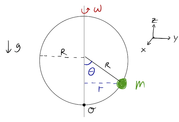
We found the equation of motion to be
\[ \begin{aligned} \ddot{\theta} = (\omega^2 \cos \theta - \frac{g}{R}) \sin \theta, \end{aligned} \]
from which we found points of equilibrium at \( \theta_{\rm eq} = 0, \pi \), and \( \cos \theta_{\rm eq} = g / (\omega^2 R) \) - where the latter two points only exist if \( \omega \) is large enough.
Let's explore the equilibrium points separately, starting with the fixed points at \( \theta_{\rm eq} = 0 \) and \( \pi \). I'll also take the condition \( \omega^2 < g/R \) for the moment, so these are the only equilibrium points.
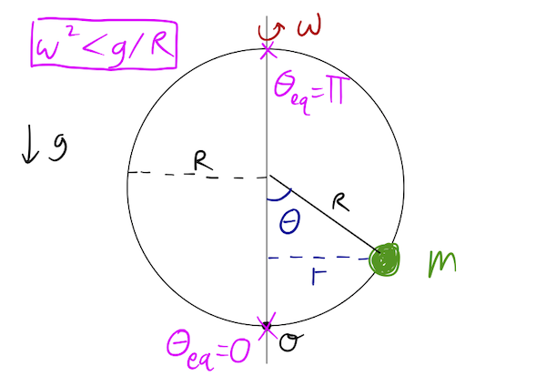
These are the "obvious" equilibrium points, at the very top and bottom of the hoop. At these points, the rotation doesn't affect the bead at all, and the force of gravity has no component along the wire, so the bead doesn't move.
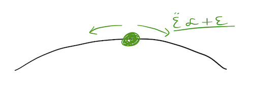
Of course, things that don't move are boring, so let's ask a more interesting question: what happens if we nudge our particle slightly away from equilibrium? To be concrete, let's consider the top point and let \( \theta = \pi + \epsilon \), where \( \epsilon \) is a small number. We can Taylor expand about the equilibrium, keeping only first-order terms:
\[ \begin{aligned} \ddot{\epsilon} = (\omega^2 \cos (\pi + \epsilon) - \frac{g}{R}) \sin (\pi + \epsilon) \end{aligned} \]
Let's recall that to Taylor expand a function around an arbitrary point, to first order we write
\[ \begin{aligned} f(x_0 + \epsilon) \approx f(x_0) + \epsilon f'(x_0) + ... \end{aligned} \]
so
\[ \begin{aligned} \cos (\pi + \epsilon) \approx \cos \pi - \epsilon \sin \pi = -1 \\ \sin (\pi + \epsilon) \approx \sin \pi + \epsilon \cos \pi = -\epsilon \end{aligned} \]
or going back,
\[ \begin{aligned} \ddot{\epsilon} \approx (\omega^2 + \frac{g}{R}) \epsilon. \end{aligned} \]
The term in parentheses is always positive, so we find that if we choose any positive \( \epsilon \), the bead will accelerate in the same direction, and the same for negative \( \epsilon \). Thus, \( \theta_{\rm eq} = \pi \) is an unstable equilibrium point. If we bump the bead slightly away from equilibrium, it will accelerate away.
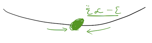
On the other hand, if we do the same exercise at the bottom of the hoop, we find that about \( \theta_{\rm eq} = 0 \), we have
\[ \begin{aligned} \ddot{\epsilon} \approx (\omega^2 - \frac{g}{R}) \epsilon. \end{aligned} \]
Given that \( \omega^2 < g/R \), the term in parentheses is always negative; whatever \( \epsilon \) we put in, the acceleration will push it in the opposite direction, back towards \( \epsilon = 0 \). This is a stable equilibrium point; if the bead is put in motion near such a point, it will stay near that point.
Notice, by the way, that this first-order equation about the stable equilibrium point is exactly the simple harmonic oscillator equation:
\[ \begin{aligned} \ddot{\epsilon} \approx (\omega^2 - \frac{g}{R}) \epsilon = - \Omega^2 \epsilon. \end{aligned} \]
So for small displacements from \( \theta=0 \), we see that the bead will oscillate back and forth with frequency
\[ \begin{aligned} \Omega = \sqrt{g/R - \omega^2}. \end{aligned} \]
An enormous number of physical systems actually behave like harmonic oscillators near their equilibrium points; this is a fairly deep point which we'll return to later in the semester.
Now, if we let \( \omega \) increase, we notice that eventually (when \( \omega^2 > g/R \)), the equilibrium at \( \theta_{\rm eq} = 0 \) becomes unstable as well! In terms of forces, the centrifugal force due to the rotation (pushing away from \( \theta=0 \)) starts to overwhelm the gravitational force (pushing towards \( \theta=0 \)) even at small \( \epsilon \), and the bead flies off.
So both equilibrium points are unstable now; does that mean the bead will just spin around in circles from any starting point? Conveniently, we can remember that as soon as this condition is met, two more equilibrium points appear along the sides of the hoop:
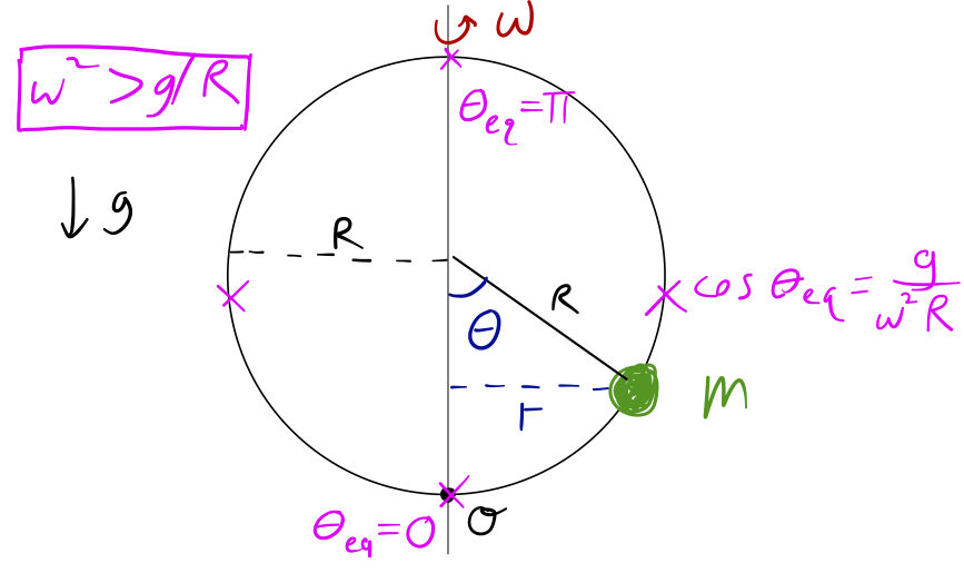
Note that since \( g / (\omega^2 R) \) is always positive, solutions only exist for \( \theta_{\rm eq} \) between 0 and \( \pi/2 \); the equilibrium points never reach the top half of the hoop. Going back to the force picture again, these are the points where gravity and centrifugal force are balanced. I leave it as an exercise to show that these two additional equilibrium points are, in fact, both stable (Taylor has the explanation, but try it yourself first!)
(If you're feeling very ambitious, here's an amusing question to think about: what happens to the equilibrium points if \( \omega^2 \) is exactly equal to \( g/R \)?)
That's all I have to say about equilibrium points for now: hopefully you can appreciate the power of this idea, and the amount of information we can learn about a system even without solving the full differential equation of motion.
Conserved quantities
By far one of the most important and fundamental theorems in physics is due to Emmy Noether. Noether was a German mathematician and physicist from the early 20th century, a time when women in either field were exceedingly rare, but she persisted in her work despite working in a challenging system, and she made a number of important contributions to mathematics and physics. Noether's theorem is stated roughly as follows:
"For any continuous symmetry of a physical system, there exists a corresponding conserved quantity."
You may have heard this statement before, but now that we're equipped with the Lagrangian, we can actually see Noether's theorem in action! In fact, we will more or less derive it very simply. (What we'll really derive is a special case of her theorem for classical systems; the general version of Noether's theorem applies even to relativistic quantum mechanics, and is immensely powerful.)
When we say that some quantity \( Q \) is conserved, in physics we just mean that it is a constant of the motion, or in other words, that \( dQ/dt = 0 \). The total energy of a system acted on by conservative forces, \( E = T + U \), is a familiar example of a conserved quantity, but far from the only possibility. In fact, we'll be able to derive the celebrated principle of conservation of energy from a simpler assumption about symmetry!
How do we see from the Lagrangian what the conserved quantities in a particular physical system are? Suppose we have a Lagrangian in some generalized coordinates, \( \mathcal{L}(q_i, \dot{q}_i, t) \). If the Lagrangian is independent of one of the coordinates, then we find:
\[ \begin{aligned} \frac{\partial \mathcal{L}}{\partial q_i} = 0 \Rightarrow \frac{d}{dt} \left( \frac{\partial \mathcal{L}}{\partial \dot{q_i}}\right) = 0. \end{aligned} \]
In other words, if the Lagrangian is independent of coordinate \( q_i \), then the quantity \( \partial \mathcal{L} / \partial \dot{q_i} \) is conserved! (Some jargon: we say the coordinate \( q_i \) which the Lagrangian doesn't depend on is a cyclic coordinate.)
But what is this derivative, physically? Well, it depends on what the coordinate \( q_i \) is. But in any case where we have a continuous symmetry, we can express it in this form, i.e. that the Lagrangian doesn't depend on the corresponding coordinate. (The rigorous version of Noether's theorem is a little more complicated and general, but this simple version is enough for the important examples we're about to see.)
Translation and rotation invariance
Let's suppose that our Lagrangian describes a single particle, and let \( q_i \) be the Cartesian coordinate \( x \). We are only allowing velocity-independent forces, so we know immediately that
\[ \begin{aligned} \frac{\partial \mathcal{L}}{\partial \dot{x}} = \frac{\partial T}{\partial \dot{x}} = m \dot{x} = p_x. \end{aligned} \]
Now, if our Lagrangian is also independent of \( x \), then the Euler-Lagrange equation tells us that
\[ \begin{aligned} \frac{\partial \mathcal{L}}{\partial x} = 0 \Rightarrow \frac{dp_x}{dt} = 0. \end{aligned} \]
This is the familiar law of conservation of momentum! There is of course nothing special about \( x \), this will work for all three Cartesian coordinates if the Lagrangian is independent of them.
What about the first part of Noether's theorem; what is the continuous symmetry of our system if \( \partial \mathcal{L} / \partial x = 0 \)? Well, if the Lagrangian is \( x \)-independent, that means we can pick up and move our physical system in \( x \), say \( x \rightarrow x + \Delta \) - note that this is a real shift, not just a change of coordinates! - and the equations of motion we find will not change at all. This symmetry is known as translation invariance.
If \( q_i \) is some other type of coordinate, we still expect to find a conserved quantity if the Lagrangian is independent of it, but we won't always find an ordinary linear momentum. Suppose we have a particle moving in two dimensions \( (x,y) \), and convert to polar coordinates \( (r,\theta) \). As we showed, the kinetic energy looks like
\[ \begin{aligned} T = \frac{1}{2} m (\dot{r}^2 + r^2 \dot{\theta}^2). \end{aligned} \]
Now if \( \partial \mathcal{L} / \partial \theta = 0 \), the symmetry is called rotational invariance. The basic idea is still that we can shift \( \theta \rightarrow \theta + \Delta \) and the physics doesn't change, but since \( \theta \) is an angle it has a different name. The resulting conserved quantity is
\[ \begin{aligned} \frac{\partial \mathcal{L}}{\partial \dot{\theta}} = mr^2 \dot{\theta}, \end{aligned} \]
which is exactly the angular momentum of the particle. You might object at this point that angular momentum in general is a vector quantity, \( \vec{L} = \vec{r} \times \vec{p} \). The same was true of the linear momentum above, of course, we were just working with components. What is conserved here is the \( \hat{\theta} \) component of \( \vec{L} \), which (since we have just a single particle rotating around the origin) is the only component; \( \vec{L}_r = \vec{r} \times (p_r \hat{r}) = 0 \). For more complicated systems the symmetry can be much more complicated to write down, but it has the same consequence; rotational invariance implies conservation of angular momentum.
More general conserved quantities
There are more exotic possibilities if our generalized coordinates are weirder, but usually we work with angles and positions, so these are the conservation laws we usually want to be aware of. For a completely arbitrary coordinate \( q_i \), the conserved quantity if the Lagrangian is invariant under changes in \( q_i \) is called the generalized momentum:
\[ \begin{aligned} p_i \equiv \frac{\partial \mathcal{L}}{\partial \dot{q_i}} \end{aligned} \]
and \( \partial \mathcal{L} / \partial q_i = 0 \) implies \( \dot{p_i} = 0 \). By the way, notice that using the generalized momentum, we can rewrite the Euler-Lagrange equation in the form
\[ \begin{aligned} \frac{\partial \mathcal{L}}{\partial q_i} = \dot{p_i}. \end{aligned} \]
As you could probably guess, the left-hand side \( \partial \mathcal{L} / \partial q_i \) is known as a generalized force, and so the E-L equation looks very similar to Newton's second law. In fact, if we pick Carteisan coordinates \( x,y,z \), it is exactly Newton's second law. We won't use generalized forces again, but we will use generalized momentum for other purposes, so remembering this relationship might help you recall what a generalized momentum looks like.
An important point in all of this is that it's not always obvious in a given coordinate system whether there is a conserved quantity or not. Consider the following Lagrangian:
\[ \begin{aligned} \mathcal{L} = \frac{1}{2} m (\dot{x}^2 + 2\dot{y}^2) + C(x-y) \end{aligned} \]
Now, obviously neither \( x \) nor \( y \) is a cyclic coordinate. However, we notice that if we apply the shift
\[ \begin{aligned} x \rightarrow x + \epsilon \\ y \rightarrow y + \epsilon \end{aligned} \]
then \( \mathcal{L} \) doesn't change at all! In more geometric terms, there is a direction in the \( xy \) plane along which our Lagrangian actually is still translation invariant. We can reveal this with a coordinate change, and then identify the conserved momentum: let's take
\[ \begin{aligned} u = x+y \\ v = x-y \end{aligned} \]
and then
\[ \begin{aligned} \dot{u} = \dot{x} + \dot{y} \\ \dot{v} = \dot{x} - \dot{y} \end{aligned} \]
Inverting, we find
\[ \begin{aligned} \dot{x} = \frac{1}{2} (\dot{u} + \dot{v}) \\ \dot{y} = \frac{1}{2} (\dot{u} - \dot{v}) \end{aligned} \]
so the kinetic energy becomes
\[ \begin{aligned} T = \frac{1}{2} m (\dot{x}^2 + 2\dot{y}^2) \\ = \frac{1}{8} m[(\dot{u}^2 + 2 \dot{u} \dot{v} + \dot{v}^2) + 2 (\dot{u}^2 - 2\dot{u} \dot{v} + \dot{v}^2) ] \\ = \frac{3}{8} m (\dot{u}^2 + \dot{v}^2) - \frac{1}{4} m\dot{u} \dot{v} \end{aligned} \]
In these coordinates, the Lagrangian is thus
\[ \begin{aligned} \mathcal{L} = \frac{3}{8} m (\dot{u}^2 + \dot{v}^2) - \frac{1}{4} m \dot{u} \dot{v} + Cv. \end{aligned} \]
Next time: we'll finish studying this example, and look for conservation of energy.