Last time, we talked about Noether's theorem and conserved quantities, which in classical mechanics (mostly) follow from a simple observation based on the Euler-Lagrange equations,
\[ \begin{aligned} \frac{\partial \mathcal{L}}{\partial q_i} = \frac{d}{dt} \left( \frac{\partial \mathcal{L}}{\partial \dot{q_i}} \right). \end{aligned} \]
If for any coordinate we have \( \partial \mathcal{L} / \partial q_i = 0 \) (this condition is also stated as "\( q_i \) is cyclic"), then the quantity \( \partial \mathcal{L}/\partial \dot{q_i} \) is conserved - it doesn't change as our system evolves.
We ended considering an example Lagrangian of the form:
\[ \begin{aligned} \mathcal{L} = \frac{1}{2} m (\dot{x}^2 + 2\dot{y}^2) + C(x-y) \end{aligned} \]
which doesn't have any obvious cyclic coordinates, but with the coordinate change
\[ \begin{aligned} u = x+y \\ v = x-y \end{aligned} \]
we can rewrite the Lagrangian as:
\[ \begin{aligned} \mathcal{L} = \frac{3}{8} m (\dot{u}^2 + \dot{v}^2) - \frac{1}{4} m \dot{u} \dot{v} + Cv. \end{aligned} \]
Clicker question
What is the conserved quantity in this Lagrangian?
A. \( u \)
B. \( v \)
C. \( m\dot{u} \)
D. \( \frac{1}{4} m (3\dot{u} - \dot{v}) \)
E. \( \frac{1}{4} m (3 \dot{v} - \dot{u}) \)
Answer: D
The coordinate \( u \) is cyclic, but it's not conserved; the corresponding conserved quantity is
\[ \begin{aligned} p_u = \frac{\partial \mathcal{L}}{\partial \dot{u}} = \frac{1}{4} m (3\dot{u} -\dot{v}). \end{aligned} \]
If we had an ordinary kinetic term, then this would just be \( m\dot{u} \), but our kinetic term became more complicated after we changed coordinates.
What do we gain by working so hard to identify a conserved quantity? Well, the big advantage is that it simplifies the time evolution greatly; rewriting our equations of motion using conserved quantities can reduce the number of equations we actually have to solve. You'll see an important example of this on the homework! As for the current problem, we can take \( \dot{u} \) and rewrite it in terms of the conserved quantity \( p_u \):
\[ \begin{aligned} \frac{4p_u}{m} = 3\dot{u} -\dot{v} \Rightarrow \dot{u} = \frac{4p_u}{3m} + \frac{1}{3} \dot{v} \end{aligned} \]
Instead of substituting into the Lagrangian, let's find the \( v \) equation of motion first, since we used the \( u \) equation of motion to find \( p_u \):
\[ \begin{aligned} \frac{\partial \mathcal{L}}{\partial v} = \frac{d}{dt} \left( \frac{\partial \mathcal{L}}{\partial \dot{v}} \right) \\ C = \frac{d}{dt} \left(\frac{3}{4} m \dot{v} - \frac{1}{4} m \dot{u}\right) \\ = \frac{d}{dt} \left(\frac{3}{4} m \dot{v} - \frac{m}{4} \left[ \frac{4p_u}{3m} + \frac{1}{3} \dot{v} \right]\right) \\ = \frac{d}{dt} \left( \frac{8}{12} m \dot{v} - \frac{p_u}{3} \right) \\ \Rightarrow \ddot{v} = \frac{3C}{2m}. \end{aligned} \]
So using our conserved quantity lets us eliminate the \( u \) variable completely, and get a single differential equation just involving \( v \)! In fact, the result is particularly simple in this case: \( p_u \) doesn't appear in our equations at all once we've done the replacement. This makes physical sense, because \( u \) and \( v \) are orthogonal coordinates, so the motion in the \( u \)-direction shouldn't do anything in the \( v \)-direction.
Note that if you just try to set \( \dot{u} = 0 \), you will get the wrong answer here! This is because for this system, \( \dot{u} \) itself is not a conserved quantity on its own.
Time translation
There's one more very important symmetry to consider, and that is time translation. This is one of the most fundamental axioms underpinning not just all of physics, but science as a whole. The idea that repeated identical experiments should have the same outcome is a critical part of the scientific method. We know from Noether's theorem that with this symmetry must come a conserved quantity, so let's try to identify it. If we have a physical system which is time-translation invariant, then in terms of the Lagrangian, we must have
\[ \begin{aligned} \frac{\partial \mathcal{L}}{\partial t} = 0. \end{aligned} \]
Yes, this is a partial derivative, not a total derivative! We don't want the entire system to be independent of time - then there's no motion to consider. We just want to ensure that there is no explicit dependence on time in \( \mathcal{L} \); the most common counterexamples would be some kind of external driving force (time dependence in \( T \)) or a time-varying electric or other force field (time dependence in \( U \).)
Above it was obvious that the Euler-Lagrange equations simplified when the derivative with respect to \( q_i \) was zero. But remember that there's also a simplification if we have a functional which doesn't depend on the independent variable, which is \( t \) here. As you showed on the first homework, the condition \( \partial \mathcal{L} / \partial t = 0 \) means that we can write the E-L equations in the second form. You only proved it for a single dependent variable, but here's what it looks like when we have multiple coordinates:
\[ \begin{aligned} \frac{d}{dt} \left(\sum_i \dot{q_i} \frac{\partial \mathcal{L}}{\partial \dot{q_i}} - \mathcal{L} \right) = 0. \end{aligned} \]
So the quantity in parentheses is our conserved quantity; it is another new function, and it is called the Hamiltonian. Recognizing the derivative as the generalized momentum, we can rewrite it:
(Definition: the Hamiltonian)
\[ \begin{aligned} \mathcal{H} = \sum_i p_i \dot{q_i} - \mathcal{L}. \end{aligned} \]
So as long as the Lagrangian does not depend explicitly on time, \( \partial \mathcal{L} / \partial t = 0 \), this new quantity is totally conserved: \( dH/dt = 0 \). What is the physical meaning of \( \mathcal{H} \)? We will explore this question a bit further later in the semester. But notice that if we start in Cartesian coordinates \( x_i \), then the kinetic energy is just \( T = \frac{1}{2} \sum_i m_i \dot{x_i}^2 \), which means that
\[ \begin{aligned} p_i = \frac{\partial \mathcal{L}}{\partial \dot{x_i}} = m_i \dot{x_i}, \end{aligned} \]
so that
\[ \begin{aligned} \sum_i p_i \dot{q_i} = \sum_i (m_i \dot{x_i} \dot{x_i}) = 2T. \end{aligned} \]
Since the Lagrangian is \( \mathcal{L} = T - U \), this means that the Hamiltonian is just
\[ \begin{aligned} \mathcal{H} = \sum_i p_i \dot{q_i} - \mathcal{L} = T + U. \end{aligned} \]
So the Hamiltonian in these coordinates is just the total energy! Time translation symmetry leads to conservation of energy as a prediction of Lagrangian mechanics. In fact, \( \mathcal{H} = T + U \) will continue to be true in any generalized coordinate system, as long as our change of coordinates doesn't depend explicitly on time, so \( \partial q_i / \partial t = 0 \). (Taylor proves this in the book, have a look at section 7.8.)
The Hamiltonian provides yet another, somewhat new way of thinking about physical systems, now in terms of momenta and positions instead of velocities and positions. In fact, we can use it to write down equations of motion and solve them: as we will prove later on, the Euler-Lagrange equations together with the definition of the generalized momentum leads us to
\[ \begin{aligned} \dot{p_i} = -\frac{\partial H}{\partial q_i} \\ \dot{q_i} = \frac{\partial H}{\partial p_i} \end{aligned} \]
These equations (Hamilton's equations) have twice as many variables, but are only first-order differential equations, which will frequently be an advantage in certain problems. However, since we just learned a new technique in the Lagrangian, we'll put off Hamiltonian mechanics until we really need it, much later in the semester.
Central Force Motion
Now we're finally going to apply the Lagrangian to solve some more complex and interesting mechanics problems. Our first stop will be what the book calls "Two-Body Central-Force Problems". As a reminder, a central force is one which is spherically symmetric; for an object moving in the force field in spherical coordinates with the source at the origin, we can write it as
\[ \begin{aligned} \vec{F}_{\textrm{cent}} = F(\vec{r}) \hat{r}, \end{aligned} \]
so the force is always directed towards or away from the source at the center. Not all forces are central; the magnetic force is an obvious counterexample. But the electric force, gravitational force, and even the force exerted by a spring are all central forces.
Moreover, these are all conservative forces, which means that they each have a corresponding potential energy function \( U \). In fact, for a central force, \( U \) must be independent of \( \theta \) and \( \phi \), otherwise the force \( \vec{F} = -\nabla U \) would end up with components in those directions. So \( U = U(r) \), and similarly \( \vec{F} = \vec{F}(r) \).
Two-body, clearly, means we will be considering problems involving only two objects. This includes a number of very interesting physical systems; the motion of a planet around the sun, and the orbit of an electron around the nucleus of an atom are the most important. Of course, the solar system contains 8 planets and a swarm of smaller objects, and most atoms have many electrons, but we can still learn a lot just by considering two objects in isolation, particularly for the solar system where the gravitational pull of the Sun dominates the effects of all of the other objects.
(The hydrogen atom is a purely two-body problem, but you'll need quantum mechanics to fully understand its properties; still, the classical setup of the two-body problem is a prerequisite for solving the quantum system.)
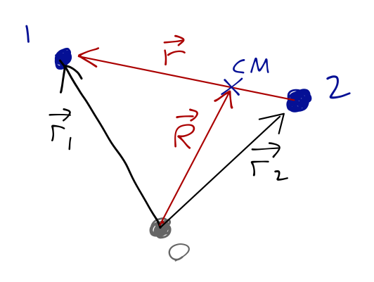
Consider two objects, labelled \( 1 \) and \( 2 \). Their masses are \( m_1, m_2 \), positions are \( \vec{r_1}, \vec{r_2} \). We assume a conservative, central force, so potential depends only on relative distance:
\[ \begin{aligned} U(\vec{r_1}, \vec{r_2}) = U(|\vec{r_1} - \vec{r_2}|) \equiv U(r). \end{aligned} \]
With all of that, the Lagrangian is
\[ \begin{aligned} \mathcal{L} = \frac{1}{2} m_1 \dot{\vec{r_1}}^2 + \frac{1}{2} m_2 \dot{\vec{r_2}}^2 - U(r). \end{aligned} \]
Now we can pick generalized coordinates! Two objects and no constraints, so we need 6. Since \( \vec{r} = \vec{r_1} - \vec{r_2} \) appears directly in the potential, we'll take its components as 3 of our GCs, so that leaves 3 more. Remember our second vector doesn't have to be orthogonal to \( \vec{r} \) in our fixed coordinates, just independent of it.
It turns out that the best choice for our remaining coordinates is the center of mass position, \( \vec{R} \):
\[ \begin{aligned} \vec{R} = \frac{m_1 \vec{r_1} + m_2 \vec{r_2}}{M}. \end{aligned} \]
\( \vec{R} \) points to the center of mass (CM), on the line joining \( m_1 \) and \( m_2 \), and \( M = m_1 + m_2 \) is the total mass.
How would you guess to use this particular coordinate? As always, you need some amount of intuition, but there are two ways we might have arrived at \( \vec{R} \):
Argue based on conservation of momentum - a collection of objects has total momentum \( \vec{P} = M \vec{R} \), and external forces act on the CM like a point particle, \( \vec{F}_{\textrm{ext}} = \dot{P} \).
Try it in the Lagrangian! Other combinations of \( \vec{r_1} \) with \( \vec{r_2} \) will give more complicated expressions.
Next time: we finish our coordinate change, and use conserved quantities to get rid of some coordinates.