Last time, we began our setup of the two-body central force problem. Our initial Lagrangian takes the form
\[ \begin{aligned} \mathcal{L} = \frac{1}{2} m_1 \dot{\vec{r_1}}^2 + \frac{1}{2} m_2 \dot{\vec{r_2}}^2 - U(r). \end{aligned} \]
The appearance of the relative distance vector \( \vec{r} = \vec{r_1} - \vec{r_2} \) in the potential suggests that we should use that as a generalized coordinate, but we counted six degrees of freedom, so we need another vector in addition to \( \vec{r} \). The best choice turns out to be the center of mass position \( \vec{R} \):
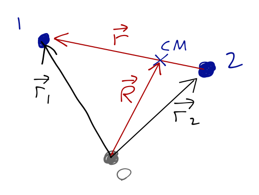
where
\[ \begin{aligned} \vec{R} = \frac{m_1 \vec{r_1} + m_2 \vec{r_2}}{M}. \end{aligned} \]
To finish our coordinate change, we need expressions for \( \vec{r_1} \) and \( \vec{r_2} \) in terms of the generalized coordinates \( \vec{r} \) and \( \vec{R} \).
Clicker Question
_What is \(r_1\) in terms of \( R \)?_
A. \( \vec{r_1} = (\vec{R} - \vec{r})/2 \)
B. \( \vec{r_1} = (\vec{R} + \vec{r})/2 \)
C. \( \vec{r_1} = \vec{R} + \frac{m_1}{M} \vec{r} \)
D. \( \vec{r_1} = \vec{R} + \frac{m_2}{M} \vec{r} \)
E. \( \vec{r_1} = \vec{R} - \frac{m_2}{M} \vec{r} \)
Answer: D
We know that \( M\vec{R} = m_1 \vec{r_1} + m_2 \vec{r_2} \), and \( \vec{r} = \vec{r_1} - \vec{r_2} \). To isolate \( \vec{r_1} \), we add \( m_2 \vec{r} \) to \( M\vec{R} \):
\[ \begin{aligned} M\vec{R} + m_2 \vec{r} = (m_1 + m_2) \vec{r_1} + (m_2 - m_2) \vec{r_2} \end{aligned} \]
Dividing both sides by \( M = m_1 + m_2 \), we arrive at answer D.
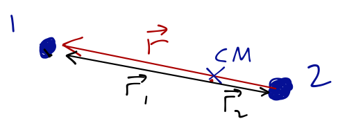
We can also argue using limits! In the limit that \( m_1 >> m_2 \), the center of mass vector should point very close to \( \vec{r}_1 \); since \( m_2 / M \rightarrow 0 \) in this limit, we narrow our choices down to D or E. Taking the opposite limit \( m_2 >> m_1 \) should give \( \vec{R} \approx \vec{r_2} \); using \( \vec{r} = \vec{r_1} - \vec{r_2} \), option D gives the correct result.
A similar construction works for \( \vec{r_2} \), so we have
\[ \begin{aligned} \vec{r_1} = \vec{R} + \frac{m_2}{M} \vec{r} \\ \vec{r_2} = \vec{R} - \frac{m_1}{M} \vec{r} \end{aligned} \]
and the kinetic energy becomes
\[ \begin{aligned} T = \frac{1}{2} m_1 \left( \dot{\vec{R}} + \frac{m_2}{M} \dot{\vec{r}}\right)^2 + \frac{1}{2} m_2\left( \dot{\vec{R}} - \frac{m_1}{M} \dot{\vec{r}}\right)^2 \end{aligned} \]
Let's simplify this. The \( \dot{\vec{R}}^2 \) terms are easy:
\[ \begin{aligned} T \supset \frac{1}{2} (m_1 + m_2) \dot{\vec{R}}^2 = \frac{1}{2} M \dot{\vec{R}}^2. \end{aligned} \]
(the \( \supset \) symbol is mathematical notation for "contains", since I'm going to simplify piece by piece.) The \( \vec{r} \cdot \vec{R} \) terms vanish:
\[ \begin{aligned} T \supset \left(\frac{m_1 m_2}{M} - \frac{m_2 m_1}{M} \right)\dot{\vec{R}} \cdot \dot{\vec{r}} = 0 \end{aligned} \]
Finally, for the \( \vec{r}^2 \) terms,
\[ \begin{aligned} T \supset \frac{1}{2} \left( \frac{m_1 m_2^2}{M^2} + \frac{m_2 m_1^2}{M^2} \right) \dot{\vec{r}}^2 = \frac{1}{2} \frac{m_1 m_2}{M} \dot{\vec{r}}^2. \end{aligned} \]
So for the Lagrangian in our GCs,
\[ \begin{aligned} \mathcal{L} = T - U = \frac{1}{2} M \dot{\vec{R}}^2 + \frac{1}{2} \mu \dot{\vec{r}}^2 - U(r) \end{aligned} \]
where I've defined the reduced mass
\[ \begin{aligned} \mu \equiv \frac{m_1 m_2}{M} = \frac{m_1 m_2}{m_1 + m_2}. \end{aligned} \]
Note that if one mass is much larger than the other, the reduced mass is almost equal to the smaller mass. For example in the Earth-Sun system, \( M \approx M_{S} \), while \( \mu \approx M_{\textrm{E}} \).
Conserved quantities in the two-body problem
Since there are no external forces, the motion of the CM (as we expect) is very simple: we have
\[ \begin{aligned} \frac{\partial \mathcal{L}}{\partial \vec{R}} = 0 \end{aligned} \]
which tells us that \( M\ddot{\vec{R}} = 0 \). Invariance under \( \vec{R} \) gives us conservation of total momentum,
\[ \begin{aligned} M \dot{\vec{R}} = \dot{\vec{P}} = \textrm{const.} \end{aligned} \]
Motion under \( \vec{R} \) is ignorable - we don't need to worry about it when solving for the dynamics of \( \vec{r} \).
In fact, from the Newtonian point of view we know that we can work in any inertial reference frame. So if we move to the CM frame in which \( \dot{\vec{R}} \) = 0, then the variable \( \vec{R} \) vanishes completely.
Are there any conserved quantities here? Since \( U \) depends only on \( |\vec{r}| \), you should suspect there are. Let's work in spherical coordinates:
\[ \begin{aligned} \mathcal{L} = \frac{1}{2} \mu \left[ \dot{r}^2 + r^2 \dot{\theta}^2 + r^2 \sin^2 \theta \dot{\phi}^2\right] - U(r). \end{aligned} \]
First, since \( \partial \mathcal{L} / \partial \phi = 0 \), we have a conserved quantity,
\[ \begin{aligned} \frac{\partial \mathcal{L}}{\partial \dot{\phi}} = \mu r^2 \sin^2 \theta \dot{\phi} = \textrm{const}. \end{aligned} \]
What is this conserved momentum? You can guess from the units that it will be some sort of angular momentum. Let's work out the total angular momentum vector of this system to see. The general formula is \( \vec{L} = \vec{r} \times \vec{p} \), and it will add for our two objects:
\[ \begin{aligned} \vec{L} = m_1 \vec{r_1} \times \dot{\vec{r_1}} + m_2 \vec{r_2} \times \dot{\vec{r_2}}. \end{aligned} \]
Now we use our coordinate change above, which is simplified by working in the CM frame: we now have \( \vec{R} = 0 \). Plugging in, we find
\[ \begin{aligned} \vec{L} = \frac{m_1 m_2^2}{M^2} \vec{r} \times \dot{\vec{r}} + \frac{m_1^2 m_2}{M^2} \vec{r} \times \dot{\vec{r}} \\ = \mu \vec{r} \times \dot{\vec{r}}. \end{aligned} \]
This result is true in any coordinate system, since it's a vector equation. If we expand out in spherical coordinates, using the standard result
\[ \begin{aligned} \dot{\vec{r}} = \dot{r} \hat{r} + r \dot{\theta} \hat{\theta} + r \sin \theta \dot{\phi} \hat{\phi}, \end{aligned} \]
(note that \( |\dot{\vec{r}}|^2 \) matches our spherical kinetic energy above!), then
\[ \begin{aligned} \vec{L} = \mu \vec{r} \times \dot{\vec{r}} = \mu \left| \begin{array}{ccc} \hat{r} & \hat{\theta} & \hat{\phi} \\ r & 0 & 0 \\ \dot{r} & r \dot{\theta} & r \sin \theta \dot{\phi} \end{array} \right| = -\mu r^2 \sin \theta \dot{\phi} \hat{\theta} + \mu r^2 \dot{\theta} \hat{\phi}. \end{aligned} \]
This doesn't quite match on to our conserved quantity, but that's partly a trick of the fact that the angular unit vectors themselves change with time in a spherical coordinate system. If you switch to a more stable Cartesian vector coordinate system, you'll find that the conserved quantity \( \partial \mathcal{L}/\partial \dot{\phi} \) that we found above is exactly \( L_z \), the \( z \)-component of this angular momentum vector.
Turning to the other angle \( \theta \), the Euler-Lagrange equation is
\[ \begin{aligned} \frac{\partial \mathcal{L}}{\partial \theta} = \frac{d}{dt} \left( \frac{\partial \mathcal{L}}{\partial \dot{\theta}} \right) \\ \mu r^2 \sin \theta \cos \theta \dot{\phi}^2 = \frac{d}{dt} \left( \mu r^2 \dot{\theta} \right). \end{aligned} \]
This is less obviously enlightening, since both sides are non-zero. But we can make progress with a clever change of coordinates. (If you're not happy with this method, you can go back to writing out the components of \( \vec{L} \) in Cartesian vector coordinates; you should find, after some painful algebra, that this condition gives you the same answer our coordinate-change argument does.)
Why should we expect another symmetry to be buried in this problem? Because the potential only depends on the distance between the two particles, \( r \); the physics should be invariant under both rotational angles. In fact, this means that we are free to rotate our coordinate system around to change the initial angle \( \theta_0 \) describing the vector \( \vec{r} \). If we choose
\[ \begin{aligned} \theta_0 = \pi/2 \end{aligned} \]
then the second Euler-Lagrange equation becomes, at \( t=0 \),
\[ \begin{aligned} 0 = \frac{d}{dt} \left(\mu r^2 \dot{\theta}\right) \end{aligned} \]
This reveals the second invariant, which is another component of angular momentum - from above, the \( L_\phi \) component in spherical coordinates. In fact, there are no free components of angular momentum left: with \( \theta0 = \pi/2 \) our other conserved quantity is \( L\theta \), and there is no \( L_r \) component. So we have found that total angular momentum \( \vec{L} \) is conserved in this system.
Now, the problem with what we've just done is that we needed \( \theta = \pi/2 \), but we only get \( \theta_0 = \pi/2 \) from our choice of coordinates; our arguments only work if \( \theta \) doesn't evolve in time. Expanding out the \( \ddot{\theta} \) equation of motion gives
\[ \begin{aligned} 0 = 2\mu r \dot{r} \dot{\theta} + \mu r^2 \ddot{\theta}, \end{aligned} \]
so everything works out as long as we do a second rotation of our coordinates to set \( \dot{\theta}_0 = 0 \) as well. We are free to do these two fixed rotations, thanks to spherical symmetry! The first puts the initial position \( \theta_0 \) of the masses in the equatorial plane, and the second rotation puts their initial velocities in the same plane.
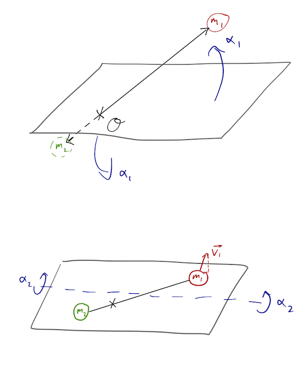
An alternative and more physical way to see the validity of this approach is to remember that \( \vec{L} = \mu \vec{r} \times \dot{\vec{r}} \). The cross product means that \( \vec{L} \) is perpendicular to both \( \vec{r} \) and \( \dot{\vec{r}} \). If \( \vec{L} \) is conserved, as we have found, then both \( \vec{r} \) and \( \dot{\vec{r}} \) lie in a fixed plane perpendicular to \( \vec{L} \). So it's valid to constrain the motion entirely to a plane.
With \( \theta \) now fixed, the only dynamical coordinates we have left are the polar coordinates \( r \) and \( \phi \). We can simplify further, since the Euler-Lagrange equation for \( \phi \) yielded a constant of the motion,
\[ \begin{aligned} \mu r^2 \dot{\phi} = L_z = \textrm{const}. \end{aligned} \]
Let's write the third and final Euler-Lagrange equation, for \( r \):
\[ \begin{aligned} \mu \ddot{r} = \mu r \dot{\phi}^2 - \frac{dU}{dr}. \end{aligned} \]
We can use \( L_z \) to substitute in to this equation for \( \dot{\phi} \), finding
\[ \begin{aligned} \mu \ddot{r} = \frac{L_z^2}{\mu r^3} - \frac{dU}{dr}. \end{aligned} \]
This is now a differential equation purely in terms of \( r(t) \). Hopefully now you can appreciate the power of finding constants of the motion! Although the dynamics of the system gives us motion in both \( r \) and \( \phi \), by identifying \( L_z \) as a constant we can reduce the problem to solving a single differential equation for \( r(t) \); once we have this, we simplify have to plug back in to the definition of \( L_z \) and integrate to find \( \phi(t) \).
Next time: we put this equation to use!