Last time, we continued our study of the two-body central force problem, and found that conservation of angular momentum forces all the motion to happen in a plane, so that we can use the two polar coordinates \( (r, \phi) \) to describe this system. Furthermore, conservation of angular momentum gives the constant of the motion
\[ \begin{aligned} \mu r^2 \dot{\phi} = L_z = \textrm{const}. \end{aligned} \]
which we can use to reduce the problem to a single differential equation for \( r \),
\[ \begin{aligned} \mu \ddot{r} = \frac{L_z^2}{\mu r^3} - \frac{dU}{dr}. \end{aligned} \]
Some more comments are in order about this equation. If there is no angular momentum, then we only have the second term, which is just the force acting in the radial direction, \( F = -\nabla U \). The extra term we have picked up can be identified as a centrifugal force term.
Notice that since the centrifugal term is just a simple power law in \( r \), it would be very easy to write it as the derivative of something. This allows us to define the effective potential
\[ \begin{aligned} U_{\textrm{eff}}(r) = U(r) + \frac{L_z^2}{2\mu r^2}, \end{aligned} \]
and then the equation of motion for \( r \) is just
\[ \begin{aligned} \mu \ddot{r} = -\frac{dU_{\textrm{eff}}}{dr}. \end{aligned} \]
Is this really still a potential energy function, though? The answer is "sort of". If we pretend that we're just solving a one-dimensional problem for a particle with mass \( \mu \) moving under the effect of \( U_{\textrm{eff}} \), then the total energy of the system is
\[ \begin{aligned} E = T + U_{\textrm{eff}} = \frac{1}{2} \mu \dot{r}^2 + \frac{L_z^2}{2\mu r^2} + U(r) \\ = \frac{1}{2} \mu \dot{r}^2 + \frac{(\mu r^2 \dot{\phi})^2}{2\mu r^2} + U(r) \\ = \frac{1}{2} \mu \dot{r}^2 + \frac{1}{2} \mu r^2 \dot{\phi}^2 + U(r) \end{aligned} \]
which is exactly the total energy from our original two-dimensional Lagrangian. In a sense, we've just pushed one of our kinetic energy terms into the potential energy for \( r \) instead. Thus, the six-dimensional motion of two objects interacting with a central force has been reduced by symmetry considerations all the way down to this equivalent one-dimensional problem.
However, there is one very important problem with interpreting \( U_{\textrm{eff}} \) as a potential energy: do not try to substitute the expression \( \mu r^2 \dot{\phi} = L_z \) into the two-dimensional Lagrangian and then solve the Euler-Lagrange equation for \( r \). You will get the wrong answer! We can only substitute for \( \dot{\phi} \) in the equations of motion, after the fact. The Lagrangian was derived assuming all the variables are independent, and solving one of the equations of motion and then trying to plug back in will not work.
In other words, it's true that \( dL_z/dt = 0 \) since it's a constant of the motion, but \( dL_z / dr \neq 0 \), and the latter will cause problems at the level of the Lagrangian. (We are done with the Lagrangian now that we have the equation for \( r(t) \), but I'm mentioning this to avoid a conceptual pitfall.)
Example: motion with no forces
In case this shuffling around of kinetic and potential energies looks suspicious to you, let's do an example with no forces at all to see what's really going on.
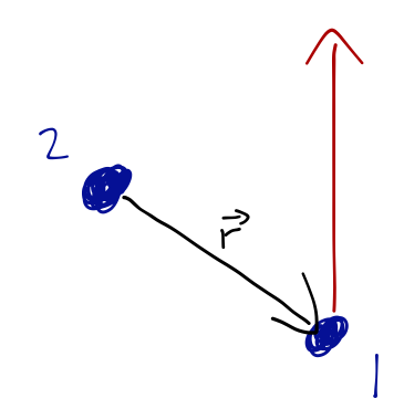
Suppose \( U = 0 \), and let's take \( m_2 \gg m_1 \) (which means \( \mu \approx m_1 \)) and look at the motion of \( m_1 \). Obviously, we know that with no forces, it will just travel past \( m_2 \) in a straight line:
Nevertheless, if we write the two-body equation of motion in our polar coordinates, we find a non-zero (effective) potential energy:
\[ \begin{aligned} U_{\textrm{eff}} = \frac{L_z^2}{2\mu r^2} \end{aligned} \]
so the equation of motion is
\[ \begin{aligned} m_1 \ddot{r} = -\frac{dU_{\textrm{eff}}}{dr} = \frac{L_z^2}{m_1 r^3}. \end{aligned} \]
Even though we started without no potential, there is an apparent "centrifugal" force! We shouldn't be surprised by this, because in fact \( r \) is a lousy coordinate for this problem. We know that \( r \) changes as the particle moves along the line; it decreases to a minimum as \( m_1 \) approaches \( m_2 \), and then starts to increase again. The equation for \( r \) is complicated because it should be! (I won't go through the solution of this differential equation for \( r(t) \), since we already know what the motion should look like.)
One more note: despite my warning above about Lagrangian substitution, remember that from the perspective of the one-dimensional problem, it's perfectly consistent to treat \( U_{\rm eff} \) as an effective potential energy. So we can write the Lagrangian as
\[ \begin{aligned} \mathcal{L} = \frac{1}{2}\mu \dot{r}^2 - \frac{L_z^2}{2\mu r^2}, \end{aligned} \]
and the equation of motion we find will be correct. What is incorrect is to start with the 2-D Lagrangian, and make this substitution:
\[ \begin{aligned} \mathcal{L} = \frac{1}{2} \mu (\dot{r}^2 + r^2 \dot{\phi}^2) \neq \frac{1}{2} \mu \dot{r}^2 + \frac{L_z^2}{2\mu r^2}, \end{aligned} \]
which clearly gives the wrong sign.
Example: spring force
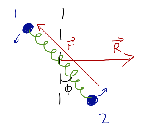
Let's do a more complete example to see everything at work here. Suppose we connect two masses \( m_1 \) and \( m_2 \) by a spring with constant \( k \) and natural length \( \ell \), and then slide them across a horizontal frictionless table: the situation is depicted below.
Before I go to the effective potential, let's consider what the two-dimensional Euler-Lagrange equations look like. They are easily seen to be:
\[ \begin{aligned} \mu \ddot{r} = \mu r \dot{\phi}^2 - k(r-\ell) \\ \mu r^2 \dot{\phi} = \textrm{const} = L_z. \end{aligned} \]
There are two special cases we can consider here. If \( L_z = 0 \) (\( \dot{\phi} = 0 \)), then the two masses are just translating but not spinning. The equation of motion becomes
\[ \begin{aligned} \mu \ddot{r} = -k(r-\ell) \end{aligned} \]
which is just the standard simple harmonic oscillator equation we would have had if the spring system was at rest. (In fact, it is at rest in the CM frame!)
What about equilibrium solutions, where \( r = \textrm{const} \)? If \( r \) is a constant then the \( \phi \) equation tells us that \( \dot{\phi} = \textrm{const} \), and from the other equation since \( \ddot{r} = 0 \) we have
\[ \begin{aligned} k(r-\ell) = \mu r \dot{\phi}^2 \end{aligned} \]
This is just "spring force = centripetal force", as the two masses revolve in simple circular motion about the CM.
After-lecture aside: what is the equilibrium value of \( r \) here? We can solve the equation to find
\[ \begin{aligned} (k - \mu \dot{\phi}^2) r = k\ell \Rightarrow r = \frac{\ell}{1 - (\mu/k) \dot{\phi}^2}. \end{aligned} \]
This is a funny-looking result, since it seems to imply that \( r \) can change signs if we spin the system fast enough! However, that's not really the case. If we begin by considering \( \dot{\phi} \) relatively small, so the denominator remains between 0 and 1, then this expression makes sense: as \( \dot{\phi} \) increases, the equilibrium value of \( r \) is pushed out towards values larger than \( \ell \), where it would be if there was no rotational motion.
However, remember that \( \dot{\phi} \) is not arbitrary here! This is not an initial condition, it's an equilibrium solution. Going back to the equation for angular momentum, we recall that
\[ \begin{aligned} \dot{\phi} = \frac{L_z}{\mu r^2}. \end{aligned} \]
So there is a stabilizing effect: as \( r \) increases, the required value of \( \dot{\phi} \) to reach equilibrium is suppressed. In fact, we can plug back in to the equation above to find the equilibrium \( r \) in terms of the angular momentum, and there will always be a solution no matter how large we make the initial \( L_z \). (The equation is a quartic polynomial so I won't try to write out the solution here, but Mathematica will give it to you if you ask nicely.)
For the more general case, the easiest way to approach the problem is in terms of the "effective potential" we defined above! For the spring, we find that
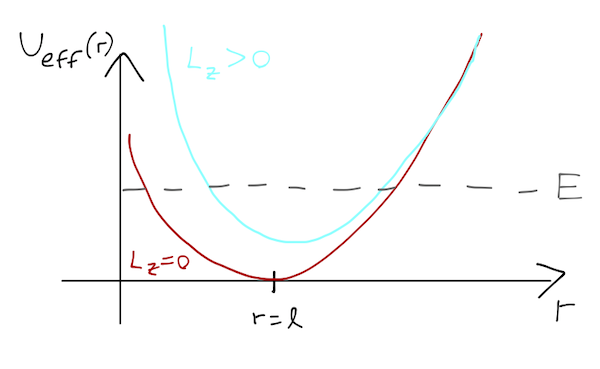
\[ \begin{aligned} U_{\textrm{eff}} = \frac{1}{2} k(r-\ell)^2 + \frac{L_z^2}{2\mu r^2}. \end{aligned} \]
So we have a quadratic term and a \( 1/r^2 \) term, which is known as the centrifugal barrier. It's easy to sketch what the shape of the potential will look like for various choices of \( L_z \):
Why is plotting \( U_{\textrm{eff}} \) useful? Remember this is completely equivalent to the 1-D problem of finding the motion of \( r \) in such a potential. Since we know total energy \( E = T + U_{\textrm{eff}} \) is conserved, we can draw lines for a given \( E \).
Whenever \( E = U_{\textrm{eff}} \), we must have \( T = 0 \), and the particle can never reach larger values of \( U \) - these are the turning points. So without solving the motion, we can see that if we start our system with greater \( E \), it will undergo oscillations with larger amplitude. For any \( E \) the particle is always "trapped"; it always has a minimum and maximum \( r \).
Clicker Question
Under what condition will the spring system always move with fixed \( r \)?
A. When \( d\phi / dt = 0 \).
B. When \( E \) takes the minimum possible value.
C. When the kinetic energy \( T = 0 \).
D. When the potential energy \( U_{\textrm{eff}} = 0 \).
E. Both B and D.
Answer: E
We can rule out answer A right away; if \( d\phi/dt = 0 \) then the spring system isn't rotating, but then we're left with a one-dimensional system of two masses connected by a spring, and away from the single equilibrium point \( r \) can definitely change in that system! (In terms of the effective potential, \( d\phi/dt = 0 \) just gives \( L_z = 0 \), and then for most values of \( E \) we see that a wide range of \( r \) are possible.)
In general, to have motion with fixed \( r \), the system must be stuck exactly at a single turning point, which means the \( E \) line must be just touching the effective potential curve; this will happen at the minimum possible \( E \). This is different from \( T=0 \), which just means that the system is at some classical turning point, and if it's only one of two turning points then \( r \) will change as the system bounces between them.
Answer D is a little trickier, but it is in fact equivalent to B. The only possible way for \( U_{\textrm{eff}} \) to be zero is if both \( r=\ell \) and \( L_z = 0 \) - but this point is precisely the minimum value of \( E \) given those conditions! So both B and D are true.
(I gave credit for B as well, because the funny thing about answer D is it corresponds to a system completely at rest - no rotation and no spring motion. So "moving with fixed \( r \)" is misleading in this case.)
The spring example doesn't turn out to be too interesting; the motion is always some sort of oscillation between minimum and maximum values of \( r \). Let's instead turn to the more interesting case of gravitational interaction. Suppose we want to solve for the motion of a comet of mass \( m \) under the influence of the Sun's gravity. The potential is
\[ \begin{aligned} U_{\textrm{eff}} = -\frac{GM_s m}{r} + \frac{L_z^2}{2\mu r^2}. \end{aligned} \]
We can sketch what this looks like, with or without angular momentum:
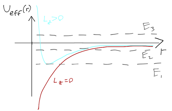
Now the motion (when \( L_z > 0 \)) is much more interesting. I've drawn three energy levels on the potential plot. \( E_1 \) corresponds to a stable, circular orbit, as in the spring example. The orbit of \( E_2 \) is also stable; there is a minimum and maximum value of \( r \), which the comet will move between in some way. Finally, \( E_3 \) is unstable; there is a minimum value of \( r \), but no maximum.
We can learn a lot just from drawing this plot and thinking about the turning points, but this approach doesn't give us the details of what is happening in the middle of the orbit. For example, we need to dig further to answer the simple question: what is the shape of an orbit with a given total energy \( E \)?
The answer is obvious if \( r \) is constant: we get a circular orbit. But if \( r \) is varying with time, just knowing the minimum and maximum possible values doesn't tell us much about what happens in the middle:
Next time: some review, and then we find the equation describing the orbital shape.