We began with review for the upcoming exam on Lagrangians - I answered any questions about the practice exam or the material in general.
More on constraints
Before we continue with central forces, I want to say a few more words about how to think about constraints when you're setting up a Lagrangian problem.
Forces of constraint
It's very important to emphasize that when we count degrees of freedom, the term "constraint" means physical constraint, i.e. constraints provided by the presence of some physical object which restricts how a dynamical system can move. As a result, for any constraint you should be able to identify a force of constraint in the Newtonian picture of a system. A few examples that we've seen:
A block resting on a table has the constraint that it can't move through the table, say \( y=0 \). The force of constraint is the normal force exerted by the table on the block.
A pendulum bob has the constraint that it remains at fixed distance \( \ell \) from the support, where \( \ell \) is the length of the string. The force of constraint is the tension from the string acting on the bob.
A bead is threaded onto a rigid wire. Although we don't usually think about it in these terms, the force of constraint here is again a normal force - one which resists any direction of motion for the bead except along the wire.
The vast majority of constraints you will encounter in Lagrangian mechanics will either correspond to normal forces or tensions. So if you're more comfortable with the force picture, it may help you to start by looking for such forces in a problem to identify the constraints for the Lagrangian approach.
An important note is that although every constraint has a force, there are many forces that do not correspond to constraints! The simplest example we've seen is a spring: a spring is not a constraint because it doesn't restrict how a system can move. Certainly the presence of a spring will change how a mass moves, but that's not the same as a restriction. If you have a mass on a spring, you're free (as an experimenter) to start with the spring compressed or stretched; but if it's also on a table, you're not free to push the mass through the table.
Of course, every force should appear somewhere in our Lagrangian solution; if it's not a force of constraint, then it must provide some contribution to the potential energy \( U \).
Ignorable coordinates vs. constraints
A concept which is sometimes confused with constraints is the idea of ignorable coordinates. For example, in the typical Atwood's machine problem, we only look at vertical motion for the blocks and assume they can't move horizontally.
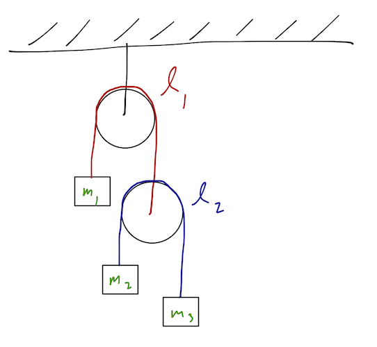
However, this is not a constraint: we know because there is no force that requires \( x_i \) to be fixed for each of the masses. Instead, the \( x_i \) are ignorable because if we solve the Euler-Lagrange equations, we find that \( \ddot{x}_i = 0 \) if the masses begin at rest and directly below the pulleys. (Again in the Newtonian picture, for this initial configuration there are no forces in the \( x \)-direction, so we know the \( x \)-accelerations will be zero.)
If you're ever in doubt about whether a coordinate is ignorable, just assume it might not be and solve the Euler-Lagrange equations in full. Ignorable coordinates are useful simplifications, but you'll never go wrong by including them!
Rolling as a constraint
Finally we come to a particularly interesting sort of constraint, which at first glance looks non-holonomic: rolling without slipping.
The condition of "rolling without slipping" is at face value a constraint on the speed: specifically, it means that the linear speed \( v \) is related to the angular speed \( \omega \) of the object,
\[ \begin{aligned} v = R \omega, \end{aligned} \]
where \( R \) is the radius. (What is the force on constraint here? It's the force of friction acting on the base of the object, specifically static friction since the contact point is instantaneously at rest.)
This is not a holonomic constraint, but there are a few special cases where we can replace it with a holonomic constraint. For example, if we have a wheel rolling down a ramp in two dimensions:
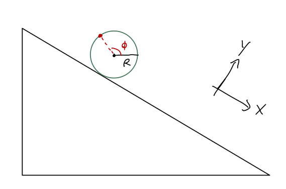
This system needs three coordinates to describe it: the usual \( x \) and \( y \), and also an angle \( \phi \) which describes the orientation of the wheel. (Imagine drawing a dot on the rim.) We have two constraints now; the wheel stays on the ramp, or \( y=0 \), and the wheel rolls without slipping, or
\[ \begin{aligned} \dot{x} = R \dot{\phi}. \end{aligned} \]
But notice that we can integrate this equation:
\[ \begin{aligned} x = R \phi + (R \phi_0). \end{aligned} \]
This is now a holonomic constraint! Because this is a relatively simple system, we can rewrite the relationship between speeds as a direct relationship between coordinates. What is the kinetic energy of the wheel? We can remember that for a rotating object, the kinetic energy is
\[ \begin{aligned} T = \frac{1}{2} I \omega^2 = \frac{1}{2} I \frac{v^2}{R^2} = \frac{1}{2} mv^2 \end{aligned} \]
where I've used \( I = mR^2 \) for a thin hoop. It just happens that we get the same formula as normal here - for example, if it was a solid disk we would find \( \frac{1}{4} mv^2 \) instead.
Unfortunately, this nice property breaks down if we try to go much further. The book gives an example involving rolling a ball around a plane, but here's another one: take the wheel and ramp, but now make the ramp an inclined plane so the problem is three-dimensional.
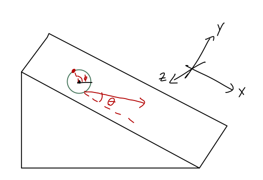
Now the wheel can rotate in two directions; about its axis as described by \( \phi \), but also relative to the direction down the plane, which we'll call \( \theta \). Now there are two conditions for rolling without slipping:
\[ \begin{aligned} \dot{x} = R\dot{\phi} \cos \theta \\ \dot{z} = R\dot{\phi} \sin \theta. \end{aligned} \]
These cannot be reduced to a simple holonomic constraint. This statement has a deeper meaning, as I've mentioned before: it means that we can't uniquely determine the orientation of the wheel (\( \theta \) and \( \phi \)) just by knowing the coordinates \( x \) and \( z \). In other words, how the wheel is oriented (and how much kinetic energy it carries!) at point \( (x,z) \) depends on which path it took to get there - not a holonomic constraint.
The equation of orbit
Back to the two-body problem. Last time, we were making use of the effective potential energy,
\[ \begin{aligned} U_{\textrm{eff}}(r) = U(r) + \frac{L_z^2}{2\mu r^2}, \end{aligned} \]
which allows us to write the equation of motion for \( r \) in the form
\[ \begin{aligned} \mu \ddot{r} = -\frac{dU_{\textrm{eff}}}{dr}. \end{aligned} \]
This defines the "equivalent one-dimensional problem", and we can use some familiar techinques like conservation of energy and turning point analysis to learn rough features of how \( r \) will evolve in time - we finished last time talking about bound and unbound orbits.
Now let's dig in further and actually find the shape of our orbital solutions. To find the shape of the orbit, our goal will be to eliminate time and solve for the function \( r(\phi) \). Let's specialize to the case of a \( 1/r \) potential now - this includes gravity and electromagnetism, so it's specific but very useful! We can write the potential as
\[ \begin{aligned} U(r) \equiv -\gamma/r. \end{aligned} \]
For gravity, \( \gamma = Gm_1 m_2 \), for electric force it would be \( -k q_1 q_2 \). Assuming this form, the EoM becomes:
\[ \begin{aligned} \mu \ddot{r} = \frac{L_z^2}{\mu r^3} - \gamma/r^{2}. \end{aligned} \]
To look for \( r(\phi) \), we trade time derivatives away using the chain rule:
\[ \begin{aligned} \frac{d}{dt} = \frac{d\phi}{dt} \frac{d}{d\phi} \\ = \dot{\phi} \frac{d}{d\phi} \\ = \frac{L_z}{\mu r^2} \frac{d}{d\phi}. \end{aligned} \]
So,
\[ \begin{aligned} \ddot{r} = \frac{d}{dt} \left(\frac{dr}{dt}\right) \\ = \frac{L_z}{\mu r^2} \frac{d}{d\phi} \left( \frac{L_z}{\mu r^2} \frac{dr}{d\phi} \right) \\ \end{aligned} \]
If we expand this out, we will get two terms, a first and a second derivative, and the equation will be messy. It would sure be nice if the thing inside the parentheses didn't depend on \( r \)...
We can fix this problem by changing variables! We want a new \( u(r) \) that will cancel the \( 1/r^2 \) when we take its derivative. In fact, what we need is
\[ \begin{aligned} u = 1/r \Rightarrow du = -1/r^2 dr, \end{aligned} \]
so that
\[ \begin{aligned} \frac{dr}{d\phi} = \frac{dr}{du} \frac{du}{d\phi} = -r^2 \frac{du}{d\phi}. \end{aligned} \]
Now life is easy:
\[ \begin{aligned} \ddot{r} = \frac{L_z}{\mu r^2} \frac{d}{d\phi} \left( -\frac{L_z}{\mu} \frac{du}{d\phi} \right) \\ = -\frac{L_z^2 u^2}{\mu^2} \frac{d^2 u}{d\phi^2}. \end{aligned} \]
Going back to the equation of motion: the right-hand side was
\[ \begin{aligned} -\frac{dU_{\textrm{eff}}}{dr} = \frac{L_z^2}{\mu r^3} - \gamma/r^{2} \\ = \frac{L_z^2 u^3}{\mu} - \gamma u^{2} \end{aligned} \]
Combining and multiplying through by \( -\mu/(u^2 L_z^2) \), we have
\[ \begin{aligned} \frac{d^2 u}{d\phi^2} = -u + \frac{\mu \gamma}{L_z^2}. \end{aligned} \]
This is almost the equation for a simple harmonic oscillator, except for the constant term. But we can absorb that easily: let
\[ \begin{aligned} w(\phi) = u(\phi) - \frac{\gamma \mu}{L_z^2}. \end{aligned} \]
Then
\[ \begin{aligned} \frac{d^2 w}{d\phi^2} = -w(\phi). \end{aligned} \]
which we know how to solve:
\[ \begin{aligned} w(\phi) = A \cos (\phi - \delta). \end{aligned} \]
We haven't specified which direction in space corresponds to \( \phi = 0 \), so we're free to choose it to get rid of the phase \( \delta \). (This assumes we're not interested in multiple two-body systems at once, e.g. for the solar system - I'll come back to this point shortly.) Then going back a step,
\[ \begin{aligned} u(\phi) = \frac{\gamma \mu}{L_z^2} + A \cos \phi. \end{aligned} \]
Finally, since \( u = 1/r \), we have for the radial coordinate
\[ \begin{aligned} r(\phi) = \frac{1}{(\gamma \mu/L_z^2) + A \cos \phi} \\ = \frac{L_z^2/(\gamma \mu)}{1 + (A L_z^2 / (\gamma \mu)) \cos \phi}. \end{aligned} \]
If I introduce two new constants:
\[ \begin{aligned} c = \frac{L_z^2}{\gamma \mu} \end{aligned} \]
and \( \epsilon = Ac \), which we take positive (we can always do this by adding a phase of \( \pi \) to \( \phi \)), then I have a fully simplified equation for \( r \):
Equation of orbit for a \( 1/r \) potential
\[ \begin{aligned} r(\phi) = \frac{c}{1+ \epsilon \cos \phi}. \end{aligned} \]
You can check that \( c \) has units of length, and \( \epsilon \) is dimensionless. It's also worth noticing that because \( A \) and \( c \) are both related to lengths, they're both positive, and so we must have \( \epsilon > 0 \).
Next time: we interpret the equation of orbit, and use it to derive some more results.