Last time, we solved for the equation of orbit describing the motion of two bodies interacting under a central force. As a reminder, we've now specialized from the general two-body problem down to a \( 1/r \) effective potential,
\[ \begin{aligned} U_{\textrm{eff}} = \frac{L_z^2}{2\mu r^2} - \frac{\gamma}{r}. \end{aligned} \]
where once again, for gravity \( \gamma = Gm_1 m_2 \). We found the equation of orbit:
\[ \begin{aligned} r(\phi) = \frac{c}{1+\epsilon \cos \phi}. \end{aligned} \]
Now that we have the equation in hand, let's try to interpret it.
An immediate and very interesting observation we can make from the equation of orbit is that \( r(\phi) \) is periodic as \( \phi \rightarrow \phi + 2\pi \). Obviously the simplest orbit occurs for \( \epsilon = 0 \), in which case we simply have
\[ \begin{aligned} r(\phi) = c, \end{aligned} \]
i.e. a circular orbit. But for more complicated orbits, this periodicity means that the orbit closes: \( r(0) \) and \( r(2\pi) \) are the same point in space. (This didn't have to be true!)
An orbit which is \( 2\pi \) periodic in \( \phi \) is called stable, since we can draw it as a simple closed curve in space. Circular orbits are always trivially stable, since they don't depend on \( \phi \).
(Fun fact: one of the key assumptions that we made to end up with a stable orbit was that the potential goes as \( U \sim 1/r \). In fact, there are only two types of potentials which give stable orbits other than circles: this, and the spring potential \( U \sim r^2 \). This fact is known as Bertrand's Law.)
Clicker Question
What is the smallest value \( r{\textrm{min}} \), and at what \( \phi \) does it occur? (Remember, \( \epsilon > 0 \)!)_
A. \( r_{\textrm{min}} = c, \phi = \pi/2 \)
B. \( r_{\textrm{min}} = c, \phi = 0 \)
C. \( r_{\textrm{min}} = \frac{c}{1+\epsilon}, \phi = \pi/2 \)
D. \( r_{\textrm{min}} = \frac{c}{1-\epsilon}, \phi = \pi \)
E. \( r_{\textrm{min}} = \frac{c}{1+\epsilon}, \phi = 0 \)
Answer: E
From the equation of orbit, it's either A, D, or E, since B and C don't work out when you plug in those values of \( \phi \). D is the minimum value of the denominator \( 1 - \epsilon \cos \phi \), but that means it's actually the maximum value of \( r \). So the answer is E, which is always less than A because \( \epsilon > 0 \).
What does this orbit look like for \( 0 < \epsilon < 1 \)? I can sketch the denominator \( c/r(\phi) \):
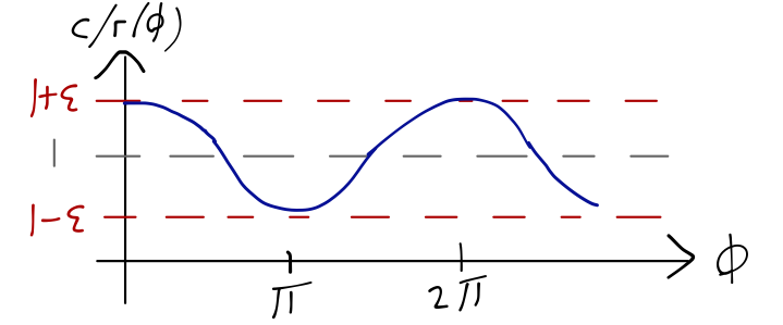
So for \( \epsilon < 1 \), we have a bound orbit, which oscillates between the values
\[ \begin{aligned} r_{\textrm{min}} = \frac{c}{1+\epsilon},\ \ r_{\textrm{max}} = \frac{c}{1-\epsilon}. \end{aligned} \]
The coordinates where minimum and maximum \( r \) occur are known as periapsis and apoapsis, respectively (remember: "a" is further away.) If the orbit is around the sun, you'll see the terms perihelion and aphelion instead; for the Earth, it's perigee and apogee.
A quick note: remember that we got rid of an arbitrary phase \( \delta \) in our derivation. We can see now that physically, the choice \( \delta = 0 \) amounts to rotating our coordinate system so that periapsis occurs at \( \phi = 0 \), on the positive \( x \)-axis. This is fine as long as we're using arbitrary coordinates, but if we have multiple two-body systems in the same coordinates (like the planets in the solar system), then we need to include the periapsis phase \( \delta \) in order to describe their motion correctly. We would do this by replacing \( \phi \) with \( \phi - \delta \) in the equation of orbit.
What does the orbit look like in space? Periapsis is at \( \phi = 0 \) and apoapsis at \( \phi = \pi \), and the radius varies smoothly between the two, so we end up with an ellipse:
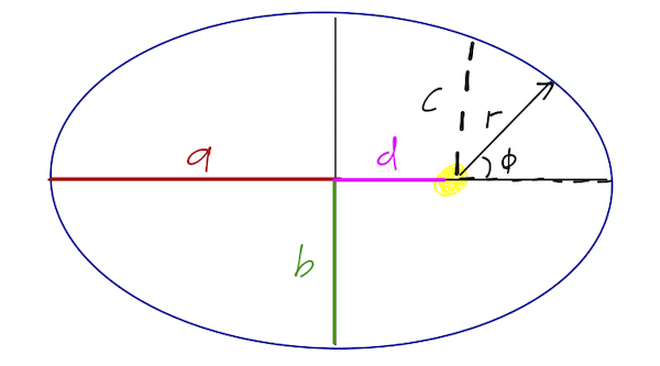
The book switches to Cartesian coordinates at this point, but I say why bother? You can already see this is an ellipse, and we can work out its properties very easily from the equation of orbit. The parameter \( \epsilon \) is called the eccentricity of the ellipse; a more eccentric orbit is more oblong. (We already saw that \( \epsilon = 0 \) is a circle.)
Just as the shape of a circle is determined by its radius, the shape of an ellipse is determined by the major and minor axes, which are like the diameter in the long and short directions. Half of the axis length is called the semimajor axis (\( a \)) or semiminor axis (\( b \)). From the equation of orbit, we can identify \( c \) on our plot as the radius at \( \phi = \pi/2 \), which means the distance to the ellipse vertically above or below the origin. Finally, I've labelled the offset between the center of the ellipse and our origin (the CM location) as \( d \).
We can write formulas for all of these lengths, but they're all easy to derive from the equation of orbit, as we will now see.
Clicker Question
What is the length \( a \), in terms of \( c \) and \( \epsilon \)?
A. \( a = c \)
B. \( a = \frac{c}{1-\epsilon} \)
C. \( a = \frac{c}{1+\epsilon} \)
D. \( a = \frac{c}{(1-\epsilon^2)} \)
E. \( a = \frac{c\epsilon}{(1-\epsilon^2)} \)
Answer: D
We know that if \( \epsilon = 0 \), we recover a circular orbit, in which case we do have \( a=c \); this eliminates choice E, which would vanish.
Geometrically, we can see that \( 2a \) is the major axis of the ellipse, which is just equal to \( r_{\rm min} + r_{\rm max} \). Thus, from the equation of orbit we find
\[ \begin{aligned} a = \frac{1}{2} (r(0) + r(\pi)) \\ = \frac{1}{2} \left( \frac{c}{1+\epsilon} + \frac{c}{1-\epsilon}\right) \\ = \frac{c}{2} \frac{1-\epsilon+1+\epsilon}{(1-\epsilon)(1+\epsilon)} \\ = \frac{c}{(1-\epsilon^2)}. \end{aligned} \]
Once we have length \( a \), it's straightforward to find \( d \) in a similar way:
\[ \begin{aligned} d = a - r_{\textrm{min}} \\ = \frac{c}{(1-\epsilon^2)} - \frac{c}{1+\epsilon} \\ = \frac{c - c + c \epsilon}{(1-\epsilon^2)} \\ = \frac{c\epsilon}{(1-\epsilon^2)} \\ = \epsilon a. \end{aligned} \]
The hardest length to find is \( b \). There are a few ways to do it: the most direct is to write the equation for a straight vertical line \( y = -d \) in polar coordinates as
\[ \begin{aligned} r \sin \phi = -d, \end{aligned} \]
and then solve for where it intersects the ellipse, and then use \( b^2 + d^2 = r^2 \). However, this is much easier if you remember a special property of an ellipse. The two points along the semimajor axis \( d \) from the center (one of which is the CM!) are called the foci of the ellipse, and any point on the ellipse is a total distance of \( 2a \) from the two foci. This is one of the definitions of an ellipse. (You can use a string of length \( 2a \) anchored at the foci to draw an ellipse, in fact.)
Because of this fact, we know that at the bottom of the ellipse,
\[ \begin{aligned} \sqrt{d^2 + b^2} + \sqrt{d^2 + b^2} = 2a \\ 4a^2 = 4(b^2 + d^2) \\ b = \sqrt{a^2 - d^2} \\ = \sqrt{a^2 - \epsilon^2 a^2} \\ = \frac{c}{\sqrt{1-\epsilon^2}}. \end{aligned} \]
Notice that the ratio of the two axes is
\[ \begin{aligned} \frac{b}{a} = \sqrt{1-\epsilon^2} \end{aligned} \]
which is another way to define an ellipse of eccentricity \( \epsilon \).
Orbital period
So now we can draw the orbit, but by going to \( r(\phi) \) we've lost information about time evolution. In particular, how do we know the orbital period, i.e. how long it takes the object to return to the starting point? Taylor does the standard "sweeping out areas" argument, but I'll show you another way using the chain rule.
We can write the orbital velocity as:
\[ \begin{aligned} \dot{r} = \frac{dr}{d\phi} \frac{d\phi}{dt} \\ = \frac{c\epsilon \sin \phi}{(1+\epsilon \cos \phi)^2} \dot{\phi} \\ = r^2 \frac{\epsilon \sin \phi}{c} \frac{L_z}{\mu r^2} \\ = \epsilon \sin \phi \sqrt{\frac{\gamma}{\mu c}}, \end{aligned} \]
remembering that \( c = L_z^2 / (\gamma \mu) \). Now, \( \dot{r} = dr/dt \), so we can reorganize into
\[ \begin{aligned} dt = dr \sqrt{\frac{\mu c}{\gamma}} \frac{1}{\epsilon \sin \phi}. \end{aligned} \]
We also know that
\[ \begin{aligned} dr = d\phi \frac{c\epsilon \sin \phi}{(1+\epsilon \cos\phi)^2} \end{aligned} \]
so combining and integrating both sides,
\[ \begin{aligned} t = \int_{\phi_i}^{\phi_f} d\phi \frac{c\epsilon \sin \phi}{(1+\epsilon \cos \phi)^2} \sqrt{\frac{\mu c}{\gamma}} \frac{1}{\epsilon \sin \phi} \\ = c^{3/2} \sqrt{\frac{\mu}{\gamma}} \int_{\phi_i}^{\phi_f} \frac{d\phi}{(1+\epsilon \cos \phi)^2}. \end{aligned} \]
Note that this is a nice expression; it will give us not just the orbital period, but the time taken for the orbit to evolve between any two angles \( \phi_i \) and \( \phi_f \). To get the orbital period, we just set the limits to \( 0 \) and \( 2\pi \). The integral takes some work, but if you do some clever substitutions or ask Mathematica nicely, you will find (for \( 0 < \epsilon < 1 \)):
\[ \begin{aligned} \tau = c^{3/2} \sqrt{\frac{\mu}{\gamma}} \frac{2\pi}{(1-\epsilon^2)^{3/2}} \end{aligned} \]
or for an object moving around the Sun under gravity, where \(\gamma = G m_1 m_2 \approx G \mu M_{\odot}\),
\[ \begin{aligned} \tau^2 = \left(\frac{c}{1-\epsilon^2}\right)^3 \frac{4\pi^2}{G M_{\odot}} = \frac{4\pi^2}{GM_\odot} a^3. \end{aligned} \]
Note: as was pointed out to me in class, this equation is often written with the sum of the solar and planet masses in the denominator. Let's see where that comes from: let \( m \) be the mass of the planet. Then the reduced mass is \( \mu = mM_{\odot} / (m + M_{\odot}) \), and we have in the orbital period formula
\[ \begin{aligned} \frac{\mu}{\gamma} = \frac{m M_{\odot}}{(m + M_{\odot}) G m M_{\odot}} = \frac{1}{G(m+M_{\odot})}, \end{aligned} \]
giving instead
\[ \begin{aligned} \tau^2 = \frac{4\pi^2}{G(m+M_{\odot})} a^3. \end{aligned} \]
which is the more correct formula.
The correction due to including \( m \) is pretty small in practice, but not always totally negligible. The mass of the Earth is about \( 3 \times 10^{-6} M_{\odot} \), so the approximate formula above gives an orbital period which is off by about 45 seconds from the correct length of a year. On the other hand, Jupiter (the heaviest planet in the solar system) has a mass of \( 0.00095 \) times \( M_{\odot} \) and a 12-year orbital period, so using \( M_{\odot} \) instead of \( m + M_{\odot} \) would give you the wrong period by 2 days. Close enough for physics homework, but if you're launching a probe to Jupiter you probably care about the difference!
We have now derived several important facts about bound orbits, and in fact, we have at this point proved all three of Kepler's Laws of planetary motion:
- Planets orbit in ellipses, with the Sun at one focus.
- Angular momentum \( L_z \) is conserved (Kepler would say this differently, "equal areas swept out in equal times".)
- The period of the orbit is given by the formula we just found.
The point I'm trying to emphasize is that from a modern point of view, Kepler's laws are all simple consequences of the two-body problem and the equation of orbit that we found. So if you remember one thing, remember that equation!
Next time: unbound orbits, and some examples.