Last time, we started to work with the equation of orbit,
\[ \begin{aligned} r(\phi) = \frac{c}{1+\epsilon \cos \phi} \end{aligned} \]
(don't forget that this is, explicitly, in a coordinate system where \( \phi = 0 \) is identified with periapsis, the point in the orbit where \( r \) is minimum.) From this we derived some results about the geometry of elliptical orbits, which occur where \( 0 \leq \epsilon < 1 \), and looked at time evolution and the orbital period.
The last result we derived was Kepler's third law,
\[ \begin{aligned} \tau^2 = \frac{4\pi^2}{G(m+M_{\odot})} a^3. \end{aligned} \]
(For any spacecraft and most planets we can totally neglect the \( m \) in the denominator - see the discussion from last lecture's notes.)
Clicker Question
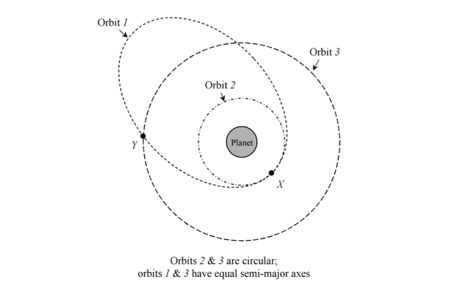
Three orbits of the same satellite are shown. Orbits 1 and 3 have the same major axis. How are their orbital periods related?
A. \( \tau_2 < \tau_1 = \tau_3 \)
B. \( \tau_2 > \tau_1 = \tau_3 \)
C. \( \tau_1 = \tau_2 < \tau_3 \)
D. \( \tau_1 = \tau_2 > \tau_3 \)
E. \( \tau_2 < \tau_1 < \tau_3 \)
Answer: A
We know that the period scales with the semi-major axis as \( \tau \propto a^{3/2} \). From the diagram, orbit 2 obviously has the shortest \( a \), while orbits 1 and 3 have identical values of \( a \) (as we're told, but you can sort of see from the picture that orbit 1 would fit within orbit 3 nicely.) So \(a_2 < a_1 = a_3\), which means that \(\tau_2 < \tau_1 = \tau_3\) - answer A.
Before we move on to \( \epsilon \geq 1 \), let's work through an example of how what we've learned so far can be applied!
Example: satellite orbit
(Note: this is actually a problem from Taylor, although I'm going to not write the number explicitly just to make it harder to find on Google for enterprising students...)
Here we consider the motion of a satellite orbiting the Earth, and we're given two facts: its closest approach to the Earth is \(r_P = 250\) km and its speed at that point is \( v = 8500 \) m/s. Can we find the eccentricity of its orbit and its furthest distance \(r_{\rm max}\)?
First of all, this is obviously a case where one object is much, much heavier, so I'll use the approximations \( \mu \approx m \) and \( m + M_e \approx M_e \), where \( m \) is the satellite mass and \( M_e \) is the Earth's mass. We have to determine \( c \) and \( \epsilon \) to know the full orbit, and we are given two quantities so that should be enough. But we need to find how the speed is determined first!
The brute-force approach would be to use the chain rule again, with the general expression \( v = \sqrt{\dot{r}^2 + r^2 \dot{\phi}^2} \) along with the equation of orbit. We'll do this shortly because it will give us a nice and general formula, but at perigee there are a couple of simpler methods we can try.
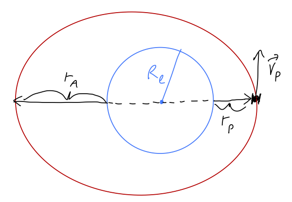
First, we can argue based on angular momentum. The direction of the velocity vector \( \vec{v} = \dot{\vec{r}} \) is always tangent to the orbit itself, and at perigee \( \vec{r} \) itself is perpendicular to the orbit:
This means that it's easy to directly evaluate the angular momentum,
\[ \begin{aligned} L_z = m|\vec{r} \times \vec{v}| = mr_{\rm min} v_P \end{aligned} \]
where \( v_P \) is the speed at perigee. (In general the cross product gives \( \sin \theta \) where \( \theta \) is the angle between the vectors, but since they're perpendicular here that's just 1.) We can plug in to the definition of \( c \):
\[ \begin{aligned} c = \frac{L_z^2}{\gamma \mu} = \frac{(m r_{\rm min} v_P)^2}{Gm^2 M_e} = \frac{r_{\rm min}^2 v_P^2}{GM_e}. \end{aligned} \]
From the sketch above, we note that \( r_{\rm min} \) is not just \( r_P \) - that's the distance above the surface of the Earth! So
\[ \begin{aligned} r_{\rm min} = r_P + R_e \approx 6650\ {\rm km}. \end{aligned} \]
We could just plug in numbers now, but as a nice little shortcut (which Taylor suggests), we can recognize that the combination \( G M_e / R_e^2 = g \), so
\[ \begin{aligned} c = \frac{r_{\rm min}^2 v_P^2}{g R_e^2} \\ = \left(\frac{6650\ {\rm km}}{6400\ {\rm km}}\right)^2 \frac{8.5\ {\rm km/s} \times 8500\ {\rm m/s}}{10\ {\rm m/s^2}} \\ = 7800\ {\rm km}. \end{aligned} \]
We can go from here directly to \( \epsilon \) through the equation of orbit:
\[ \begin{aligned} r_{\rm min} = \frac{c}{1+\epsilon} \\ \epsilon = \frac{c}{r_{\rm min}} - 1 = \frac{7800\ {\rm km}}{6650\ {\rm km}} - 1 = 0.17. \end{aligned} \]
Finally, we can use this to find the distance above the Earth's surface at apogee:
\[ \begin{aligned} r_{\rm max} = \frac{c}{1-\epsilon} = \frac{7800\ {\rm km}}{0.83} = 9400\ {\rm km} \\ r_{A} = r_{\rm max} - r_e = 3000\ {\rm km}. \end{aligned} \]
Unbound orbits
Let's come back to the case \( \epsilon \geq 1 \), which should be perfectly good solutions - our equation of orbit derivation only required that \( \epsilon \geq 0 \). Let's start at the boundary, with \( \epsilon = 1 \). Then the orbit is
\[ \begin{aligned} r(\phi) = \frac{c}{1+\cos \phi}. \end{aligned} \]
Again, closest approach is still at \( \phi = 0 \) by construction, but now we see a divergence: the radius becomes infinite at \( \phi = \pm \pi \). This must be an unbound orbit; the two objects can escape each other completely (infinite separation.)
What sort of shape is this? It's easier to see in Cartesian coordinates. We know that \( x = r \cos \phi \), so
\[ \begin{aligned} r = \frac{c}{1+x/r} \\ = \frac{cr}{r+x} \\ r+x = c \\ r^2 = (c-x)^2 = c^2 - 2cx + x^2 \\ x^2 + y^2 = c^2 - 2cx + x^2 \\ x = \frac{c}{2} - \frac{y^2}{2c}. \end{aligned} \]
This is a parabola, opening to the left along the \( x \)-axis; the closest approach is at \( r_{\rm min} = c/2 \).
If we continue to increase \( \epsilon \) beyond 1, the radius goes to infinity for angles \( \phi < \pi \). We can switch to Cartesian coordinates in a similar way, but it's messier. I won't go through the algebra, but I'll simply tell you these curves are now hyperbolas.
A hyperbola looks similar to a parabola, but it has asymptotes, lines which it will never cross. This is actually one feature of conic sections that's much easier to see in polar coordinates! The angles of the asymptotic lines are easy to read off of the equation of orbit:
\[ \begin{aligned} \cos (\phi_{\textrm{max}}) = \pm 1/\epsilon. \end{aligned} \]
In other words, if you draw a ray from the origin along a direction given by an angle greater than \( \phi_{\rm max} \), it will never cross the hyperbolic orbit. For a parabolic orbit, this isn't true; the parabola crosses every line that isn't the \( x \)-axis itself away from \( r_{\rm min} \).
The point of closest approach is, as always, at \( r_{\textrm{min}} = c/(1+\epsilon) \). We can sketch the set of all orbits, bound and unbound, that we've found:
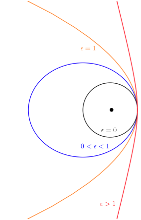
From this picture, we find an intuitive connection back to where our discussion of orbits started, namely the orbital energy. Clearly, as \( \epsilon \) increases so does the energy of the moving object; its apoapsis point moves outwards to less negative maximum values of the gravitational potential. We can confirm this intuition by going back to our energy diagram:
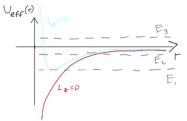
Now we can remember that circular orbits have the minimum possible energy, bound orbits (the ellipses) always have \( E < 0 \), and finally unbound orbits occur for \( E \geq 0 \); thus, the parabolic orbit with \( \epsilon = 1 \) must have \( E = 0 \) as well.
But how exactly does \( E \) depend on the parameters of the orbit? Let's go back to the equation of orbit once again, and try to be more quantitative.
Orbital energy and angular momentum
Given a particular force law and pair of objects, the length \( c \) is determined entirely by the angular momentum \( L_z \):
\[ \begin{aligned} c = \frac{L_z^2}{\gamma \mu}. \end{aligned} \]
We can reverse this equation to find
\[ \begin{aligned} L_z = \sqrt{\gamma \mu c} \end{aligned} \]
or for the specific case of gravity,
\[ \begin{aligned} L_z = \sqrt{Gm_1 m_2 \mu c} \\ \approx \mu \sqrt{GMc} \end{aligned} \]
in the usual limit where one mass is much larger than the other, so \( m_1 \approx \mu \) and \( m_2 \approx M \). So, angular momentum (per unit mass) goes as the square root of the length \( c \).
What about energy? We know at the turning points that the kinetic energy vanishes, so \( E = U_{\textrm{eff}} \). Let's work at \( r_{\textrm{min}} \), which is the only turning point which exists for both bound and unbound orbits:
\[ \begin{aligned} E = U_{\textrm{eff}} (r_{\textrm{min}}) = - \frac{\gamma}{r_{\textrm{min}}} + \frac{L_z^2}{2\mu r_{\textrm{min}}^2} \\ = \frac{1}{2r_{\textrm{min}}} \left( \frac{L_z^2}{\mu r_{\textrm{min}}} - 2\gamma\right). \end{aligned} \]
From above we know that
\[ \begin{aligned} r_{\textrm{min}} = \frac{c}{1+\epsilon} = \frac{L_z^2}{\gamma \mu (1+\epsilon)}, \end{aligned} \]
so
\[ \begin{aligned} E = \frac{\gamma \mu (1+\epsilon)}{2L_z^2} \left( \gamma (1+\epsilon) - 2\gamma\right) \\ = \frac{\gamma^2 \mu}{2L_z^2} (\epsilon^2 - 1). \end{aligned} \]
The coefficient out front here is always positive. This matches our expectations; for \( 0 \leq \epsilon < 1 \), \( E < 0 \) and the orbit is bound (and is a circle or ellipse.)
We can re-express this more geometrically by substituting back in for the angular momentum \( L_z^2 = \gamma \mu c \):
\[ \begin{aligned} E = \frac{\gamma}{2c} (\epsilon^2 - 1) \end{aligned} \]
or explicitly for a bound orbit,
\[ \begin{aligned} E = -\frac{\gamma}{2a}. \end{aligned} \]
We know this version has to be only valid for bound orbits, for two reasons: one, since \( \gamma \) and \( a \) are both positive this formula always gives a negative energy; and two, for an unbound orbit \( a \) (defined using the distance \( r_{\rm max} \)) doesn't exist!
For gravity in the limit where one mass is much smaller than the other, we can substitute in to find
\[ \begin{aligned} E = \frac{GM\mu}{2c} (\epsilon^2 - 1) \\ = \frac{-GM\mu}{2a}. \end{aligned} \]
Next: we'll finish with orbital speed, and do some more examples.