Before we wrap up with orbital mechanics and gravity, there are a couple more applications I want to briefly talk about.
Flyby assists
Also known as the gravitational slingshot! This is an application of unbound orbits, regularly used by NASA to speed up trips to the outer solar system.
For a flyby assist described by an unbound orbit, the important thing to note here is that the incoming and outgoing speed are identical, so \( v_i = v_f \). We could have guessed this from the start, because the interaction with a planet conserves total energy \( E \). So how is this an assist? Consider a hyperbolic orbit of a spacecraft around Venus:
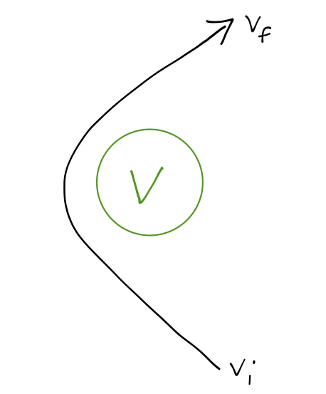
Although the final speed is unchanged in the planet-spacecraft system, the direction of the velocity vector changes - and this change of direction does give an increased speed in another frame of reference, that of the Sun! If we consider the motion relative to the Sun, we have to add the relative velocity of the spacecraft to the velocity of the planet it's flying by (Venus, in this example):
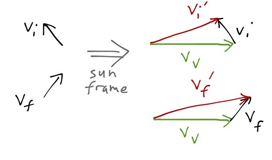
Clearly this can be used to slow down as well as speed up. There's no problem with energy conservation - the spacecraft is taking energy from (or giving energy to) the flyby planet.
This technique is used very frequently by NASA. The Voyager missions launched in the 1980's partly because of a rare alignment of the large outer planets - Jupiter, Saturn, Uranus, and Neptune. A series of flyby assists helped Voyagers 1 and 2 to make it all the way to Neptune in about 10 years after their launch in 1977 - it would have taken 30 years otherwise! The flyby assists helped Voyager 2 to overtake Pioneer 10 and 11, deep-space probes which were launched several years earlier.
Orbital transfers
As we've seen, we can compare the energy and angular momentum of different orbits at a glance based on the length scales \( a \) and \( c \). This comparison is particularly important if we want to change orbits, like moving from a low-Earth orbit to a higher one, or sending an arriving probe into a stable orbit around Mars.
Let's see quantitatively what happens to the orbit when we apply a tangential thrust - an instantaneous change in speed in the direction of motion. Suppose we start in an elliptical orbit and boost at periapsis:
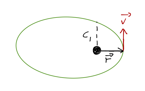
We write the new speed as \( v_2 = \lambda v_1 \); \( \lambda \) is the thrust factor. Before boosting, the orbit is described by the equation of orbit,
\[ \begin{aligned} r_1 = \frac{c_1}{1 + \epsilon_1 \cos \phi}. \end{aligned} \]
The new orbit is described by the same equation:
\[ \begin{aligned} r_2 = \frac{c_2}{1+\epsilon_2 \cos (\phi - \delta)} \end{aligned} \]
Notice that a phase shift \( \delta \) has reappeared! We threw this away when solving for a single orbit, by insisting that periapsis (closest approach) is at \( \phi = 0 \). But now we've fixed our coordinates using orbit 1, and we're not guaranteed that orbit 2 has periapsis at the same point! So we have to include \( \delta \).
We can narrow our options down; since \( \vec{v} \) and \( \vec{r} \) are perpendicular before we boost, and the boost doesn't change the direction, they stay perpendicular. This means that the new orbit is either at periapsis or apoapsis, so \( \delta = 0, \pi \).
Changing \( v \) means changing angular momentum; remember, \( c \propto L_z^2 \). This means that
\[ \begin{aligned} c_2 = \lambda^2 c_1. \end{aligned} \]
We can use this and equate the two orbits at the point of the boost \( \phi = 0 \) in order to solve for \( \epsilon_2 \); I'll skip over this because the resulting equation isn't very enlightening, but if you do this in practice it's important to keep track of all your plus and minus signs, including the one that can appear if \( \delta = \pi \). Boosts at apoapsis follow the same approach, just with \( \phi = \pi \).
We can combine orbital thrusts to change from one central-force orbit to another; this is great for e.g. going between planets in the Solar system. The most energy-efficient way to accomplish this orbital change is the Hohmann transfer, which is an elliptical orbit with periapsis and apoapsis at the two planets to be transferred between.
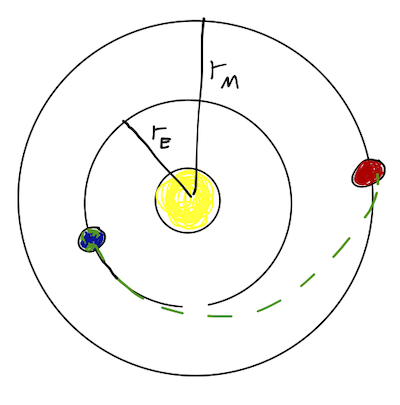
To execute this maneuver we have to thrust forwards, at both departure at arrival! We can make sense of this in terms of energy: the semimajor axes satisfy \( a_E < a < a_M \) for the three orbits in succession, and since \( E \propto -1/a \), we are increasing total energy towards \( E=0 \) as \( a \) increases. (To go the other way, from Earth to Mars, then we would have to decelerate twice.)
Restricted three-body problem
You might worry that our treatment of the two-body problem has been a bit too restrictive; it's fine for dealing with a single planet orbiting the Sun, but what about the moons orbiting those planets, or satellites moving through the Solar System?
The moment we have more than two bodies interacting, this entire framework we've built up goes out the window, even if there are only central forces. But we can solve a restricted three-body problem by making some big assumptions.
The restricted three-body problem is very complicated and difficult, although you now know enough about central force motion and Lagrangian mechanics to understand how to solve it. I'll just give you the high points in lecture. If you're interested in knowing more, many classical mechanics textbooks treat the full restricted three-body problem (although mainly graduate-level books.)
Here are the restrictions: we assume one mass is much, much smaller than the others: \( m_3 \ll m_1, m_2 \). Also, we assume \( m_1, m_2 \) are in a circular orbit. I'll also continue to assume the motion is planar. These are strong assumptions, but close enough to describe the motion of a space probe in the Earth-Sun system, say. With that context in mind, we'll choose gravity as our central force as well.
In a circular orbit, the angular speed of \( m_1 \) and \( m_2 \) is:
\[ \begin{aligned} \dot{\phi} = \frac{L_z}{\mu r^2} = \frac{\sqrt{\gamma \mu c}}{\mu r^2}. \end{aligned} \]
For this orbit, \( c = r \) and \( \gamma = G \mu M \), so we find
\[ \begin{aligned} \dot{\phi}^2 \equiv \omega^2 = \frac{G(m_1 + m_2)}{r^3}. \end{aligned} \]
We can think of these masses generating a time-dependent gravitational potential for \( m_3 \), because of their mutual rotation. But it's much easier to deal with a static potential, so instead let's change coordinates to a rotating frame in which \( m_1 \) and \( m_2 \) are stationary.
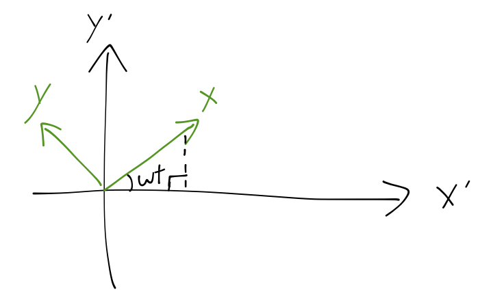
The \( x, y \) coordinates in this frame are related to the stationary ones \( x', y' \) as
\[ \begin{aligned} x = x' \cos \omega t + y' \sin \omega t\\ y = y' \cos \omega t - x' \sin \omega t. \end{aligned} \]
After some algebra, this gives a relatively nice-looking kinetic energy:
\[ \begin{aligned} T = \frac{1}{2} m_3 (\dot{x'}^2 + \dot{y'}^2) = \frac{1}{2} m_3 \left[ (\dot{x} - \omega y)^2 + (\dot{y} + \omega x)^2\right]. \end{aligned} \]
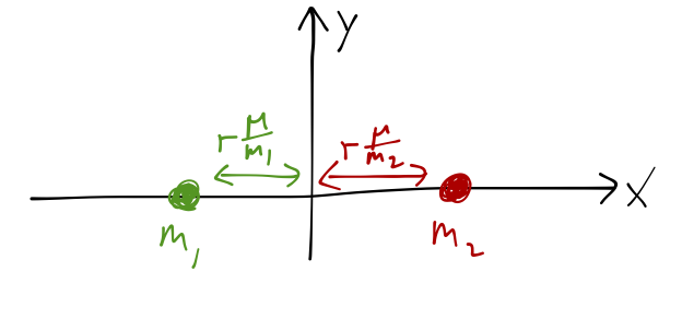
The potential is just given by the distances between \( m_3 \) and the other masses,
\[ \begin{aligned} U = \frac{-Gm_1 m_3}{r_{13}} - \frac{Gm_2 m_3}{r_{23}} \\ = \frac{-Gm_1m_3}{\sqrt{(x+r\mu/m_1)^2 + y^2}} - \frac{Gm_2 m_3}{\sqrt{(x-r\mu/m_2)^2 + y^2}}, \end{aligned} \]
using the definition of the center of mass. Writing \( \mathcal{L} = T - U \) and going through some more algebra, the equations of motion turn out to be
\[ \begin{aligned} m_3 \ddot{x} = 2 m_3 \omega \dot{y} + m_3 \omega^2 x - \frac{dU}{dx} \\ m_3 \ddot{y} = -2 m_3 \omega \dot{x} + m_3 \omega^2 y - \frac{dU}{dy}. \end{aligned} \]
These are really difficult equations to solve, as you might guess. The motion is so complex that it is actually chaotic in general - infinitesmal changes in the initial conditions can completely change the trajectory. But we can at least solve for points of equilibrium where \( \dot{x} = \dot{y} = \ddot{x} = \ddot{y} = 0 \).
I won't do this on the board, because we'd be here for a while, so I'll skip to the answer; five equilibrium points appear from these equations of motion, known as the Lagrange points, \( L_1 \) through \( L_5 \):
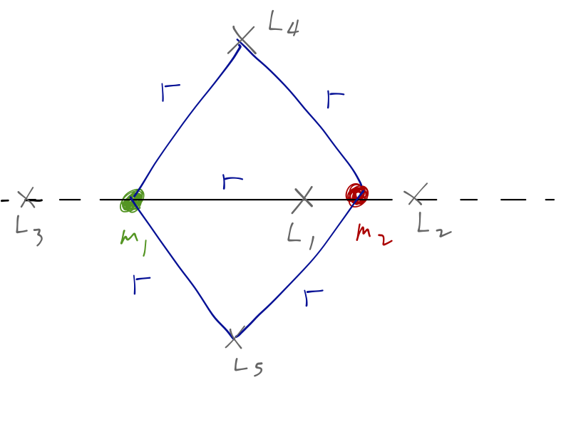
For a planet moving around the Sun, \( r \) is roughly the orbital distance, so \( L_4 \) and \( L_5 \) are on the planet's orbital path, ahead of and behind it.
We could go further to study small oscillations around the Lagrange points; we would find \( L_4 \) and \( L_5 \) to be stable equilbria, while the other three are unstable. There tends to be an accumulation of debris at \( L_4 \) and \( L_5 \) for this reason; some other planets (Jupiter, Mars) actually have large asteroids trapped at their \( L_4 \) and \( L_5 \) points. These asteroids are known as "trojans." (Jupiter has a lot of trojan asteroids, and when early astronomers saw two clusters of asteroids gathered on opposite sides of the planet, they named them all after characters in the Trojan War - Greeks on one side, Trojans on the other.)
NASA often makes use of the Lagrange points for spacecraft, allowing for long missions with minimal energy use. Solar observatories for example are best placed at \( L_3 \) (no moon to get in the way.) Observatories looking out into the universe (like the WMAP and PLANCK satellites observing the cosmic microwave background) sit at \( L_2 \) in the Earth's shadow.
Frames with linear acceleration
We've spent a lot of time on Lagrangian mechanics, but today we begin to study mechanics in non-inertial reference frames - frames which are accelerating in one way or another (linear acceleration, or rotation of any kind.)
Lagrangian mechanics lets us deal with these frames - we've done it before - but we still must start in an inertial frame of reference before changing to generalized coordinates within the non-inertial frame.
In many cases, it's easier and more intuitive to start within an accelerating frame; the good news is that it's not so difficult! Newton's laws actually can be fixed up to hold in accelerating frames, too; we just have to include some extra "fictitious forces" coming from the acceleration. Despite the name, to an observer in an accelerating frame, the forces are completely real and measurable, as you know if you've ever been in a car or an airplane. (In fact, we can in principle make use of the effects we're about to discuss to decide whether we're in an accelerating frame experimentally, without any other information.)
Let's start with a simple physical example to see how acceleration might look in different frames of reference. Suppose we have a cart containing an air cannon, that shoots a ping pong ball straight up into the air:
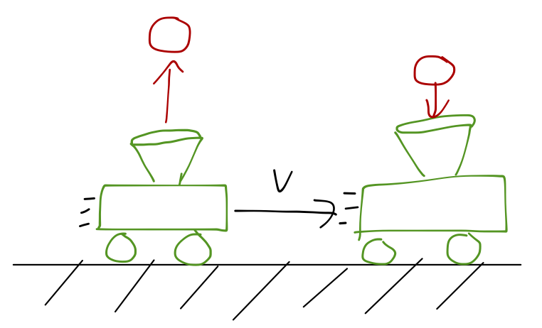
If the cart is at rest, then the ball goes up and comes straight back down, and the cart catches it. Of course, you know that the exact same thing happens if the cart is moving with constant speed, \( v \): the horizontal component of the velocity \( v_x \) is identical for the ball and the cart, so it catches the ball again.
In the latter case, to an observer on the cart, the cart is in fact stationary, and it's obvious that the ball will come back to its starting point. The cart observer's frame of reference is inertial, since the cart has constant speed, so Newton's laws are just as valid for them.
Now, what if the cart is accelerating forward with constant acceleration \( a \)? Where does the ball land?
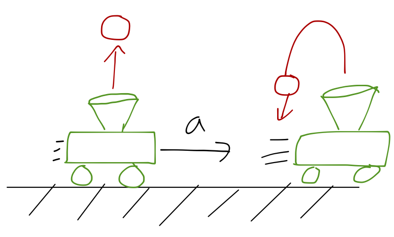
Well, to an outside observer it's perfectly obvious; the cart accelerates horizontally, the ball does not, so the cart moves out from under the ball and the ball lands behind the cart. But in the frame of reference of an observer on the cart, it looks like the ball is pushed backwards; like there's some sort of force acting on the ball to accelerate it away from the cart.
Let's see exactly what's going on in terms of forces, first in our inertial frame \( \mathcal{S}_1 \), and then in the cart frame \( \mathcal{S}_2 \). In \( \mathcal{S}_1 \), we know that Newton's laws are valid, i.e.
\[ \begin{aligned} m \ddot{\vec{r_1}} = \vec{F}. \end{aligned} \]
where \( \vec{r_1} \) is the position of the ball in \( \mathcal{S}_1 \). \( \vec{F} \) is just the net sum of familiar forces; gravity, the force exerted on the ball by the cart's air cannon, air resistance, etc. We know how to tally them all and solve for the ball's acceleration.
Once we've solved for the motion of the ball in \( \mathcal{S}_1 \), we know how to describe it in \( \mathcal{S}_2 \) as well. If the difference in velocity between the two frames is \( \vec{v} \), then the velocity-addition formula applies:
\[ \begin{aligned} \dot{\vec{r_1}} = \dot{\vec{r_2}} + \vec{v}. \end{aligned} \]
In words, the velocity of the ball relative to the ground is the velocity relative to the cart, plus the velocity of the cart relative to the ground. Taking the time derivative, we see that
\[ \begin{aligned} \ddot{\vec{r_1}} = \ddot{\vec{r_2}} + \vec{a} \end{aligned} \]
We can plug this back into Newton's law above:
\[ \begin{aligned} m \ddot{\vec{r_2}} = \vec{F} - m \vec{a}. \end{aligned} \]
This is almost Newton's second law, but with an extra term due to the acceleration of \( \mathcal{S}_2 \). In fact, to the observer in the cart frame, it looks like Newton's laws do apply, but there is one extra force compared to what the ground observer sees, namely
\[ \begin{aligned} \vec{F}_{\textrm{inertial}} = -m \vec{a}. \end{aligned} \]
This apparent force is opposite the direction of the acceleration. You've probably observed this personally: if you've ever been on a bus that brakes suddenly, you know that you get pushed forwards by the sudden stop.
Let's see a practical example of using this fictitious force.
Example: pendulum in an accelerating car
Back to the Newtonian approach! A pendulum of length \( \ell \) and mass \( m \) is attached to the ceiling of a boxcar, which is accelerating with constant acceleration \( \vec{a} \) to the right.
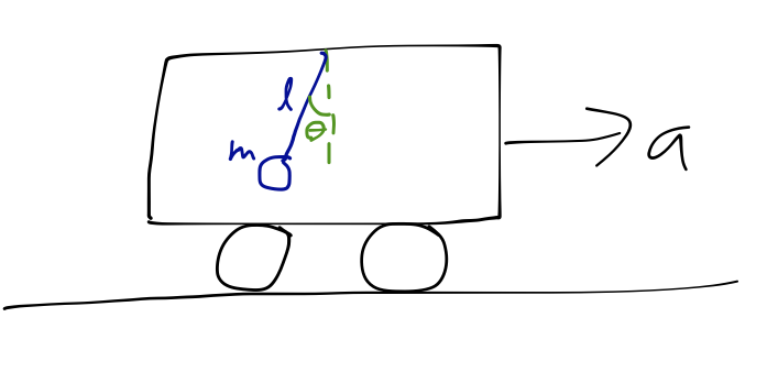
Let's draw the free-body diagram for the pendulum bob within the accelerating frame. We know that the usual forces of tension and gravity are acting on it, but now we have to include the fictitious inertial force as well:
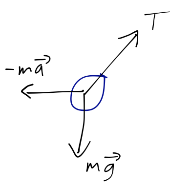
Since gravity and the inertial force are both proportional to mass, we can actually combine them as
\[ \begin{aligned} m\vec{g} - m\vec{a} \equiv m \vec{g_{\textrm{eff}}}, \end{aligned} \]
defining the effective gravitational force.
Next time: we'll finish this problem, and move on to rotation.