Last time, we saw how to modify Newton's laws in a linearly accelerating frame. The modification was very simple: we just have to add a "fictitious" inertial force,
\[ \begin{aligned} \vec{F}_{\textrm{inertial}} = -m\vec{a}. \end{aligned} \]
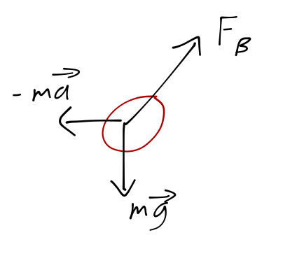
This is just adding a constant vector, since the whole frame is accelerating together in a single direction. We started doing an example of a pendulum in an accelerating boxcar:
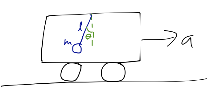
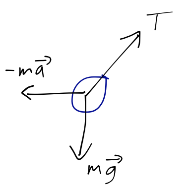
and sketched the free-body diagram:
It's been awhile since you've last used force vectors and Newton's laws, so how about a little practice?
Clicker Question
What is the equilibrium angle of the pendulum?
A. \( \phi_{\rm eq} = \sqrt{g^2 + a^2} / a \)
B. \( \phi_{\rm eq} = \sqrt{g^2 + a^2} / g \)
C. \( \phi_{\rm eq} = \sin^{-1} (a/g) \)
D. \( \phi_{\rm eq} = \tan^{-1} (g/a) \)
E. \( \phi_{\rm eq} = \tan^{-1} (a/g) \)
Answer: E
At equilibrium, the forces will be balanced, which means the tension \( T \) will satsify the two equations
\[ \begin{aligned} T \sin \phi = ma \\ T \cos \phi = mg \end{aligned} \]
Dividing the two equations by each other, we have
\[ \begin{aligned} \tan \phi = a/g \end{aligned} \]
which is answer E.
We can also skip straight to computing \( \vec{g_{\textrm{eff}}} \equiv \vec{g} - \vec{a} \), which will point in the direction \( \tan^{-1} (a/g) \), immediately giving us the equilibrium angle. All of this is much simpler than doing everything in full using the Lagrangian - sometimes forces are convenient!
We can even keep going to find the frequency of small oscillations without too much trouble. If we displace a small distance from equilibrium, the restoring force is \( mg_{\textrm{eff}} \sin (\phi - \phi_{\textrm{eq}}) \):
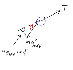
which gives the usual equation of motion for a pendulum,
\[ \begin{aligned} m (\ddot{\theta} \ell) = -mg_{\textrm{eff}} \sin (\phi - \phi_{\textrm{eq}}) \\ \ddot{\phi'} = -\frac{g_{\textrm{eff}}}{\ell} \sin \phi' \end{aligned} \]
where I've replaced \( \phi' = \phi - \phi_{\textrm{eq}} \) to make this look exactly like the equation for a simple pendulum. So we can just read off the frequency of small oscillations:
\[ \begin{aligned} \omega = \sqrt{g_{\textrm{eff}}/\ell} = \sqrt{\frac{\sqrt{g^2 + a^2}}{\ell}}. \end{aligned} \]
Here's a fun variant of this question: suppose instead of a pendulum, we tie a helium balloon to the bottom of the accelerating car.
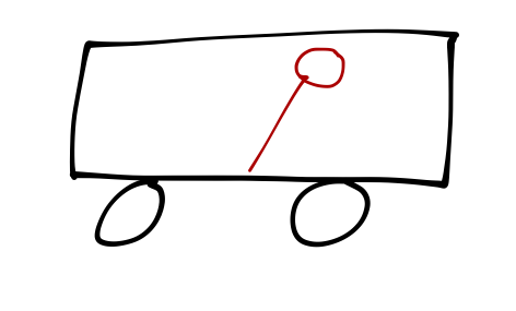
Which way does it tilt at equilibrium? You might guess to the left, since the inertial force pushes in that direction. But the balloon is also subject to buoyant force - and the inertial force pushes on the air as well as the balloon! This creates a horizontal pressure gradient, so the normally upwards-pointing buoyant force now points to the right:
The buoyant force overcomes both gravity and the external acceleration, and so the balloon tilts to the right, with the motion of the car. (This isn't completely obvious - to really figure this out we'd need the tools to actually calculate what the buoyant force is.)
There's a similar effect to watch out for when considering friction in accelerating frames, which you'll explore on this week's homework. The thing to remember is that kinetic friction acts to oppose the relative motion of two surfaces, so be careful if one of your surfaces is accelerating!
Rotating frames
Rotation is another example of acceleration which is a bit more complicated to deal with. If I take the same boxcar from last time and spin it around the center instead:
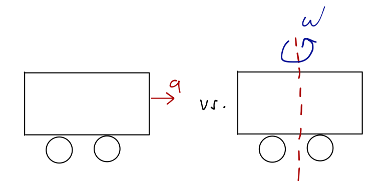
now the system is still accelerating, but the acceleration varies depending on where I stand inside the boxcar.
Rotation is also much more important, because we live on the Earth and the Earth is rotating! It would be very inconvenient to have to do every calculation in our lab frame by first starting in a fixed inertial frame and accounting for the spinning of the Earth. Of course, since you didn't do this in your freshman labs, you should suspect that the violations of Newton's laws due to the Earth's rotation aren't so big, but it's certainly important to know exactly what the effects are and what their magnitude is.
Let's set up some useful formalism, before we go on to derive the fictitious forces.
Quick math review: cross products
Since we'll be seeing a lot more cross products in the near future, we'll begin with a brief review. The cross product \( \vec{A} \times \vec{B} \) of two vectors \( \vec{A} \) and \( \vec{B} \) is another vector which is perpendicular to both \( \vec{A} \) and \( \vec{B} \). Since any two distinct vectors define a plane, the direction of \( \vec{A} \times \vec{B} \) is unique up to a sign. The magnitude of the cross product is
\[ \begin{aligned} |\vec{A} \times \vec{B}| = AB \sin \theta, \end{aligned} \]
where \( \theta \) is the opening angle between \( \vec{A} \) and \( \vec{B} \). Note that the cross product of any vector with itself is zero (since \( \theta \) is zero.) Don't forget that order matters in the cross product: flipping the vectors gives back a minus sign,
\[ \begin{aligned} \vec{A} \times \vec{B} = -\vec{B} \times \vec{A} \end{aligned} \]
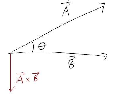
All that's left is to determine the sign, which is in fact a convention - we're free to choose which way the positive cross-product points. We will follow the standard physics convention, which is the right-hand rule: if you hold out your right hand with the thumb pointing in the direction of \( \vec{A} \) and your fingers in the direction of \( \vec{B} \), then your palm points in the direction of \( \vec{A} \times \vec{B} \). Try it with my diagram above!
The right-hand rule can be stated in terms of the Cartesian basis vectors as
\[ \begin{aligned} \hat{x} \times \hat{y} = \hat{z} \\ \hat{y} \times \hat{z} = \hat{x} \\ \hat{z} \times \hat{x} = \hat{y}. \end{aligned} \]
This is only one choice of convention, and not three; the "right-hand rule" applies independent of which two axes you point your thumb and fingers along, in other words. An easy way to remember these three equations without using your hand is that the last two equations are cyclic permutations of the first: that is, rearrangements of the three vectors that preserves the order from left to right. We can write the same identity for any set of three basis vectors, for example in cylindrincal coordinates \( \hat{r} \times \hat{\phi} = \hat{z} \), and so on.
Knowing how the cross product acts on the basis vectors, we can expand out the cross product in components. The shorthand way to remember how the components expand out is to write the cross product as a three-by-three matrix determinant,
\[ \begin{aligned} \vec{A} \times \vec{B} = \left|\begin{array}{ccc} \hat{x}&\hat{y}&\hat{z}\\ A_x&A_y&A_z\\ B_x&B_y&B_z\end{array}\right| \\ = (A_y B_z - A_z B_y) \hat{x} - (A_x B_z - A_z B_x) \hat{y} + (A_x B_y - A_y B_x) \hat{z}. \end{aligned} \]
(We'll see determinants again later on in the course. If you're not really comfortable with using them at this point, just expand each vector in components and use the basis vector cross products above.)
Two more very useful identities are known as the triple products: first, the scalar triple product, which satisfies
\[ \begin{aligned} \vec{A} \cdot (\vec{B} \times \vec{C}) = \vec{B} \cdot (\vec{C} \times \vec{A}) = \vec{C} \cdot (\vec{A} \times \vec{B}) \end{aligned} \]
(cyclic permutation again!) This isn't a full treatment, just a review, so I'll just remind you that the scalar triple product has a geometric interpretation as the volume of a parallelepiped defined by the three vectors in the product. In the volume interpretation, it's easy to see that the three products defined here should all be equal: they're just three different choices of which side of the solid we call the "base".
Next, the vector triple product lets us simplify combinations of cross products:
\[ \begin{aligned} \vec{A} \times (\vec{B} \times \vec{C}) = \vec{B} (\vec{A} \cdot \vec{C}) - \vec{C} (\vec{A} \cdot \vec{B}); \end{aligned} \]
Taylor gives this identity the mnemonic "BAC-CAB rule". You can think of this as the distribution rule for cross products, which becomes a dot product with each of the two vectors in the parentheses, times the other vector (and with an important minus sign.)
We can keep going and define more and more complicated identities, but I'll just give one more which we'll actually put to use shortly. Taking the modulus of a cross product gives a result in terms of dot products:
\[ \begin{aligned} |\vec{A} \times \vec{B}|^2 = |\vec{A}|^2 |\vec{B}|^2 - (\vec{A} \cdot \vec{B})^2. \end{aligned} \]
(This sometimes carries the name "Lagrange's Identity" - as if he didn't have enough things named after him already!)
Clicker Question
\( \vec{u} \) points down, and \( \vec{v} \) points out of the page. Which way does \( \vec{u} \times \vec{v} \) point?
A. Left
B. Right
C. Into the page
D. Up
Answer: A
Just apply the right-hand rule!
(Aside: you've probably seen the "dots and crosses" notation for vectors into/out of the page many times before. If you haven't, think of the vector as an arrow - the kind you use with a bow. If the arrow is facing out of the page, you see the point; into the page, you see the feathers.)
Clicker Question
Consider the following vector:
\[ \begin{aligned} \vec{A} = 3 \hat{x} - 2\hat{y} + \hat{z} \end{aligned} \]
Calculate \( \vec{A} \times \hat{z} \).
A. \( 3\hat{y} + 2\hat{x} \)
B. \( 3\hat{y} - 2\hat{x} \)
C. \( 3\hat{y} - 2\hat{z} + \hat{x} \)
D. \( -3\hat{y} - 2\hat{x} + \hat{x} \)
E. \( -3\hat{y} - 2\hat{x} \)
Answer: E
From above, the products of the other unit vectors with \( \hat{z} \) are
\[ \begin{aligned} \hat{y} \times \hat{z} = \hat{x} \\ \hat{z} \times \hat{x} = \hat{y}, \end{aligned} \]
where the latter equation of course implies that \( \hat{x} \times \hat{z} = -\hat{y} \). Accounting for the extra sign, we arrive at option A.
We could also have done this using the determinant formula:
\[ \begin{aligned} \vec{A} \times \hat{z} = \left|\begin{array}{ccc} \hat{x}&\hat{y}&\hat{z}\\ 3&-2&0\\ 0&0&1\end{array}\right| \\ = \hat{x} \left| \begin{array}{cc} -2 & 0 \\ 0 & 1 \end{array} \right| - \hat{y} \left| \begin{array}{cc} 3 & 0 \\ 0 & 1 \end{array} \right| \\ = -2\hat{x} - 3\hat{y}. \end{aligned} \]
This didn't save us much time here, but only because I gave you relatively simple vectors; usually the determinant trick is much quicker than multiplying out every combination of unit vectors.
The angular velocity vector
Back to physics, and to rotation! Recall that rotation involves a rigid body or collection of bodies spinning about an axis. So we need a magnitude (angular velocity, \( \omega \)) and a direction (symmetry axis). We can combine these into a vector! If the symmetry axis is \( \hat{u} \) (for unit), then
\[ \begin{aligned} \vec{\omega} = \omega \hat{u}. \end{aligned} \]
Along a given axis, \( \vec{\omega} \) can point up or down. But rotation can also be clockwise or counter-clockwise; so the direction of \( \vec{\omega} \) is meaningful. We have to pick a convention! Once again we use the standard right-hand rule convention (the "other right-hand rule"): point your right thumb in the direction of \( \vec{\omega} \), and your fingers curl in the direction of the rotation.
.)](https://physicscourses.colorado.edu/phys3210/phys3210_sp20/images/fig-RHR-wikipedia.png)
For \( \vec{\omega} \) pointing up, the rotation is thus counter-clockwise. For an object rotating around the origin, what is the relation between \( \vec{\omega} \) and the ordinary velocity \( \vec{v} \)?
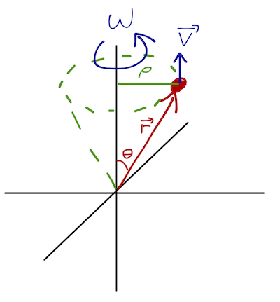
We know the linear speed is
\[ \begin{aligned} v = \rho \omega = (r \sin \theta) \omega, \end{aligned} \]
and \( \hat{v} \) is directed into the page. This of course looks like a cross product; all we have to do is make sure we get the sign right! Based on the sketch, applying the first "right-hand rule" for vector cross products, we can see that we obtain the correct direction for \( \vec{v} \) by choosing
\[ \begin{aligned} \vec{v} = \vec{\omega} \times \vec{r}. \end{aligned} \]
Time derivatives and rotating frames
Notice that we can rewrite our equation for linear speed as
\[ \begin{aligned} \dot{\vec{r}} = \vec{\omega} \times \vec{r}. \end{aligned} \]
In other words, taking the cross product with \( \omega \) gives the time derivative of \( \vec{r} \). There's nothing special about \( \vec{r} \) in this equation; it's actually true for any vector, as we will now see. Let's use a coordinate system where \( z \) points along \( \vec{\omega} \), and \( x, y \) are coordinates which are fixed with respect to the rotation.
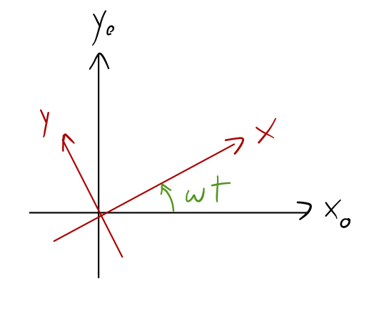
We'll call the rotating frame \( \mathcal{S} \), with coordinates \( (x,y,z) \), and also consider a fixed, inertial frame \( \mathcal{S}_0 \), coordinates \( (x_0, y_0, z_0) \). At \( t=0 \), they are identical, and of course \( z = z_0 \) since the rotation is about that axis. Working in the fixed coordinates, we can write one set of unit vectors in terms of the other:
\[ \begin{aligned} \hat{x} = \hat{x_0} \cos \omega t + \hat{y_0} \sin \omega t\\ \hat{y} = \hat{y_0} \cos \omega t - \hat{x_0} \sin \omega t. \end{aligned} \]
So if I have a vector which appears to be stationary in my rotating coordinate system,
\[ \begin{aligned} \vec{Q} = Q_x \hat{x} + Q_y \hat{y} + Q_z \hat{z} \end{aligned} \]
with all components satisfying \( dQ_i/dt = 0 \), then in the fixed coordinates, what I see is
\[ \begin{aligned} \vec{Q} = (Q_x \cos \omega t - Q_y \sin \omega t) \hat{x_0} + (Q_x \sin \omega t + Q_y \cos \omega t) \hat{y_0} + Q_z \hat{z_0}. \end{aligned} \]
How does \( \vec{Q} \) vary with time in the stationary frame \( \mathcal{S}_0 \)? Ignoring the fixed \( \hat{z}_0 \) component, we find
\[ \begin{aligned} \left(\frac{d\vec{Q}}{dt}\right)_{\mathcal{S_0}} = (-\omega Q_x \sin \omega t - \omega Q_y \cos \omega t) \hat{x_0} + (\omega Q_x \cos \omega t - \omega Q_y \sin \omega t) \hat{y_0} \\ = \omega (\vec{z_0} \times \vec{Q}) \\ = \vec{\omega} \times \vec{Q}, \end{aligned} \]
where the subscript reminds us that we're taking the derivative in the fixed frame \( \mathcal{S}_0 \).
Next time: we'll put our newly-derived forces to work with some examples (and a return of the Lagrangian!)