Last time, we started to study rotating frames of reference, and with the following setup:
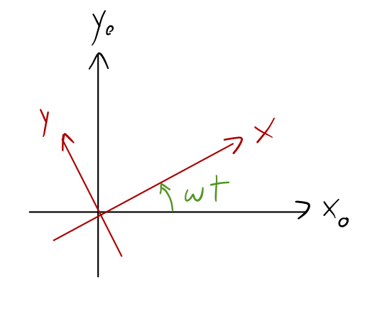
we found that for a vector \( \vec{Q} \) which is stationary in the rotating frame \( \mathcal{S} \), its time dependence in stationary frame \( \mathcal{S}_0 \) is given by the formula
\[ \begin{aligned} \left(\frac{d\vec{Q}}{dt}\right)_{\mathcal{S_0}} = \vec{\omega} \times \vec{Q}. \end{aligned} \]
What if \( \vec{Q} \) depends on time in the rotating frame, i.e. \( (d\vec{Q}/dt)_{\mathcal{S}} \neq 0 \)? Things don't change much! In the rotating coordinates, we have
\[ \begin{aligned} (d\vec{Q}/dt)_{\mathcal{S}} = \dot{Q_x} \hat{x} + \dot{Q_y} \hat{y} + \dot{Q_z} \hat{z}. \end{aligned} \]
What about the derivative in \( \mathcal{S}_0 \)? Let's look at the \( \hat{x}_0 \) component and apply the chain rule:
\[ \begin{aligned} (d\vec{Q}/dt)_{\mathcal{S}_0,x} = \frac{d}{dt} \left(Q_x \cos \omega t - Q_y \sin \omega t \right) \hat{x_0} \\ = \left[ (\dot{Q_x} \cos \omega t - \dot{Q_y} \sin \omega t) + (-\omega Q_x \sin \omega t - \omega Q_y \cos \omega t)\right] \hat{x_0}. \end{aligned} \]
The first term here is exactly how the (x-component of) \( (d\vec{Q}/dt)_{\mathcal{S}} \) looks in the fixed coordinates \( \mathcal{S}_0 \)! We find a similar result for the other two components, which means that in general,
Time derivative of a vector in a rotating frame
\[ \begin{aligned} \left( \frac{d\vec{Q}}{dt}\right)_{\mathcal{S}_0} = \left( \frac{d\vec{Q}}{dt}\right)_{\mathcal{S}} + \vec{\omega} \times \vec{Q}. \end{aligned} \]
You can remember this as something like another velocity-addition rule; the motion of \( \vec{Q} \) that we see in the inertial frame \( (d\vec{Q}/dt)_{\mathcal{S}0} \) is equal to its motion relative to the rotating frame \( (d\vec{Q}/dt){\mathcal{S}} \), plus the motion of the rotating frame relative to the inertial frame, \( \vec{\omega} \times \vec{Q} \).
Now we're ready to tackle Newton's second law, much like we did for linear acceleration.
Newton's Second Law in a Rotating Frame
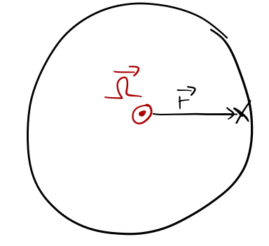
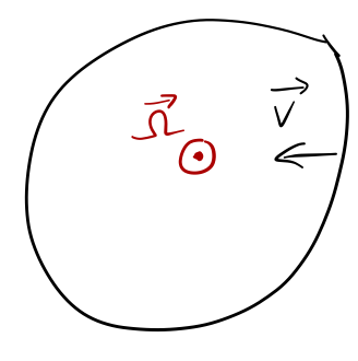
Here I'll switch notation as the book does, and use capital \( \vec{\Omega} \) to represent the relative angular velocity of \( \mathcal{S} \). This reminds us that \( \Omega \) is a special vector related to changing frames; we could still have some angular motion represented by an \( \omega \) within the rotating frame.
As before, start with Newton's 2nd law in the fixed frame:
\[ \begin{aligned} m \left(\frac{d^2 \vec{r}}{dt^2} \right)_{\mathcal{S}_0} = \vec{F}. \end{aligned} \]
Now we start rewriting the derivatives, using the relation we just found.
\[ \begin{aligned} \left(\frac{d^2 \vec{r}}{dt^2} \right)_{\mathcal{S}_0} = \left(\frac{d}{dt}\right)_{\mathcal{S}_0} \left(\frac{d\vec{r}}{dt} \right)_{\mathcal{S}_0} \\ = \left(\frac{d}{dt}\right)_{\mathcal{S}_0} \left[ \left( \frac{d\vec{r}}{dt}\right)_{\mathcal{S}} + \vec{\Omega} \times \vec{r} \right] \\ = \left(\frac{d}{dt}\right)_{\mathcal{S}} \left[ \left( \frac{d\vec{r}}{dt}\right)_{\mathcal{S}} + \vec{\Omega} \times \vec{r} \right] + \vec{\Omega} \times \left[ \left( \frac{d\vec{r}}{dt}\right)_{\mathcal{S}} + \vec{\Omega} \times \vec{r} \right]. \end{aligned} \]
All the time derivatives are now in frame \( \mathcal{S} \) which is our destination, so let's go back to dot notation. Expanding the first term gives us
\[ \begin{aligned} \left(\frac{d}{dt}\right)_{\mathcal{S}} \left[ \dot{\vec{r}} + \vec{\Omega} \times \vec{r} \right] = \ddot{\vec{r}} + \dot{\vec{\Omega}} \times \vec{r} + \vec{\Omega} \times \dot{\vec{r}} \end{aligned} \]
and the second term gives
\[ \begin{aligned} \vec{\Omega} \times \left[ \dot{\vec{r}} + \vec{\Omega} \times \vec{r} \right] = \vec{\Omega} \times \dot{\vec{r}} + \vec{\Omega} \times (\vec{\Omega} \times \vec{r}). \end{aligned} \]
Plugging back into Newton's second law above and moving all of the new terms over to the other side, we reverse some of the cross products (remember: \( \vec{A} \times \vec{B} = -\vec{B} \times \vec{A} \).) So we have finally:
Equation: fictitious forces in a rotating frame
\[ \begin{aligned} m \ddot{\vec{r}} = \vec{F} + 2m \dot{\vec{r}} \times \vec{\Omega} + m (\vec{\Omega} \times \vec{r}) \times \vec{\Omega} + m \vec{r} \times \dot{\vec{\Omega}} \\ = \vec{F} + \vec{F}_{\textrm{cor}} + \vec{F}_{\textrm{cf}} + \vec{F}_{\textrm{Euler}}. \end{aligned} \]
As promised, this is more complicated than linear acceleration - we have three fictitious forces to worry about:
- Centrifugal force:
\[ \begin{aligned} \vec{F}_{\rm cf} = m (\vec{\Omega} \times \vec{r}) \times \vec{\Omega} \end{aligned} \]
- Coriolis force:
\[ \begin{aligned} \vec{F}_{\rm cor} = 2m \dot{\vec{r}} \times \vec{\Omega} \end{aligned} \]
- Euler force:
\[ \begin{aligned} \vec{F}_{\rm Euler} = m \vec{r} \times \dot{\vec{\Omega}} \end{aligned} \]
By the way, we could have just as easily derived all of these fictitious forces by way of the Lagrangian approach instead! We know in frame \( \mathcal{S}_0 \), the Lagrangian is given by
\[ \begin{aligned} \mathcal{L} = \frac{1}{2} mv^2 - U(\vec{r}) = \frac{1}{2} m \left|\left( \frac{d\vec{r}}{dt}\right)_{\mathcal{S}_0}\right|^2 - U(\vec{r}) \end{aligned} \]
so, substituting the derivative just as we did above, the Lagrangian in frame \( \mathcal{S} \) is just
\[ \begin{aligned} \mathcal{L} = \frac{1}{2}m |\dot{\vec{r}} + \vec{\Omega} \times \vec{r}|^2 - U(\vec{r}). \end{aligned} \]
The Euler-Lagrange equation for \( \vec{r} \) will then give us exactly the same set of fictitious forces (as you will see on the next homework assignment!)
Let's start to get a feeling for these rotational forces by considering a simple example.
Example: the merry-go-round
Our example is a merry-go-round: a simple, circular platform which is rotating at some angular speed \( \Omega \). Let's take the rotation to be counter-clockwise, so \( \vec{\Omega} = \Omega \hat{z} \). Because we're looking at motion on a two-dimensional surface which is perpendicular to the motion, i.e. \( \vec{r} \) and \( \vec{\Omega} \) are always perpendicular, the dynamics will be simplified somewhat.
Suppose we're sitting on the merry-go-round at \( \vec{r} = r\hat{x} \), and \( \vec{\Omega} \) is in the \( +\hat{z} \) direction. Let's start with the centrifugal force.
We start with the general expression:
\[ \begin{aligned} \vec{F}_{\rm cf} = m (\vec{\Omega} \times \vec{r}) \times \vec{\Omega} \end{aligned} \]
To evaluate this, we apply the RHR - carefully! First, the vector \( \vec{\Omega} \times \vec{r} \) is tangential to the motion, pointing in the \( +\hat{y} \) direction. So \( (\vec{\Omega} \times \vec{r} ) \times \vec{\Omega} \) points outwards, the \( +\hat{x} \) direction. This is, of course, just opposite the direction of the centripetal acceleration which is applied in a stationary external frame to keep us moving in a circle.
Another way to see the direction is through one of the cross-product identities we wrote out last time:
\[ \begin{aligned} (\vec{\Omega} \times \vec{r}) \times \vec{\Omega} = \vec{r} (\vec{\Omega} \cdot \vec{\Omega}) - \vec{\Omega} (\vec{\Omega} \cdot \vec{r}). \end{aligned} \]
Since in this case \( \vec{\Omega} \cdot \vec{r} = 0 \), the force is in the \( \vec{r} \) direction; moreover, we can see easily that its magnitude is
\[ \begin{aligned} |\vec{F}_{\rm cf}| = m \Omega^2 r. \end{aligned} \]
Actually, we can use this same vector identity to step back and find a more general insight about the centrifugal force. Forget the merry-go-round for a moment, and suppose that \( \vec{\Omega} \) and \( \vec{r} \) are completely general. As long as we orient our coordinate system so that \( \vec{\Omega} = \Omega \hat{z} \), then
\[ \begin{aligned} \vec{r} (\vec{\Omega} \cdot \vec{\Omega}) - \vec{\Omega} (\vec{\Omega} \cdot \vec{r}) = \Omega^2 (r_x \hat{x} + r_y \hat{y} + r_z \hat{z}) - \Omega^2 r_z \hat{z} \\ = \Omega^2 (r_x \hat{x} + r_y \hat{y}) \\ = \Omega^2 \vec{\rho}, \end{aligned} \]
where \( \vec{\rho} \) is the radius in cylindrical coordinates. So (again, if \( \vec{\Omega} = \Omega \hat{z} \)),
\[ \begin{aligned} \vec{F}_{\textrm{cf}} = m \Omega^2 \rho \hat{\rho}. \end{aligned} \]
Centrifugal force is always directed radially outwards from the axis of rotation! This should match your intuition, of course, but it's good to see it coming out of the math.
Clicker Question
Now you start to walk in the \( -\hat{x} \) direction. Which way does the Coriolis force \( \vec{F}{\textrm{cor}} \) point?_
A. \( +\hat{x} \)
B. \( -\hat{x} \)
C. \( +\hat{y} \)
D. \( -\hat{y} \)
Answer: C
Using \(\vec{F}_{\rm cor} = 2m \dot{\vec{r}} \times \vec{\Omega}\), with \( \dot{\vec{r}} \) in the \( -\hat{x} \) direction, and \( \Omega \) in the \( +\hat{z} \) direction, the RHR gives \( +\hat{y} \) for the direction of the Coriolis force.
Finally, the Euler force will only appear when the ride is starting or stopping, i.e. when some angular acceleration is applied. If you return to your seat at \( +\hat{x} \) on the merry-go-round, you will feel the Euler force when the ride ends, and a \( \dot{\vec{\Omega}} \) vector appears (in the \( -\hat{z} \) direction - can you see why?) The Euler force is then directed in the \( +\hat{y} \) direction, pushing you forwards (it's a backwards force when the ride starts.)
Let's do a more involved (but still qualitative) example, again in a plane perpendicular to the rotation, to improve our intuition for looking in two different frames.
Example: "orbit" on a turntable
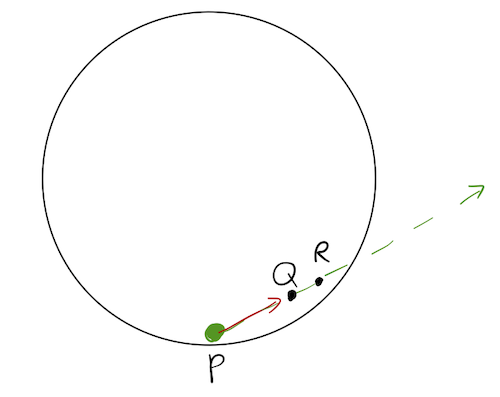
Consider an air-hockey puck, moving on the surface of a frictionless turntable. The turntable is rotating at constant angular speed \( \omega \), but we don't know the direction (yet.) We are standing on the turntable, and when we release the puck with initial speed \( v_0 \), we observe this trajectory:
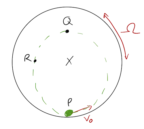
So the puck appears to follow an "orbit", and comes back to point P. Let's try to break down the motion. We know that there are only two forces in play here: the centrifugal force and Coriolis force (no Euler force since \( \vec{\Omega} \) is constant.)
\[ \begin{aligned} \vec{F}_{\rm cf} = m(\vec{\Omega} \times \vec{r}) \times \vec{\Omega} \\ \vec{F}_{\rm cor} = 2m \dot{\vec{r}} \times \vec{\Omega} \end{aligned} \]
Actually, we can simplify the centrifugal force again since \( \vec{r} \) is in a plane perpendicular to \( \vec{\Omega} \):
\[ \begin{aligned} \vec{F}_{\rm cf} = m \Omega^2 \vec{r}. \end{aligned} \]
How do they combine to give us the trajectory shown? Let's start at point Q, the turning point of the orbit:
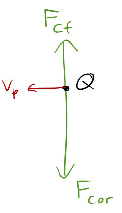
Since Q is above the center, the centrifugal force has to be pointing up, away from the center. But for the puck to turn around as we observe, the net force at Q must be towards the center, which tells us that the Coriolis force is pointing the other way.
Thanks to this information, we now have experimental evidence for which way the turntable is rotating! Since \( F_{\rm cor} \) is pointing down at Q, while \( \vec{v} \) is to the left, the rotation must be clockwise, i.e. \( \vec{\Omega} \) points into the page (\( -\hat{z} \) direction.)
Knowing the direction of rotation, we can move on to consider the forces at other points, like R:
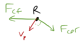
Here the centrifugal force points to the left, and the Coriolis force down and to the right. We don't know the magnitude precisely, but we can see the effect on the speed of the puck; since \( F_{\rm cor} \) is perpendicular to the velocity vector it doesn't cause any change in speed. On the other hand, \( F_{\rm cf} \) has a component in the direction of motion, so we see the puck is speeding up in the rotating frame at R. If we look on the other side of the center, we'll see it's slowing down.
One more important realization is that although the motion looks rather complicated in the rotating frame, we should remember that it's always equally valid to step back to the lab frame and look at the problem in a different way. What does our "orbit" look like in the lab frame?
Yes, it's simply a straight line! It has to be a straight line, because in the inertial lab frame, all the fictitious forces disappear, and there are no other forces in this problem. Points P, Q and R are all simply rotating around, intersecting the straight-line trajectory of the puck at different times.
Note that this was a bit of a tricky question; there's no actual "orbital" motion here. Although the puck returns to point P, it only does so once, before flying off the table entirely! Returning to point P also, clearly, requires a very specific choice of \( v_0 \) relative to \( \Omega \).
This lab-frame picture should emphasize to you that there really isn't anything mysterious about the fictitious rotational forces, even if they look strange and intimidating. The centrifugal force is very familiar; it exactly corresponds with the centripetal acceleration, which is provided to keep an object moving in a circular path.
The Coriolis effect, as we've seen, is nothing more than what happens when something is moving in a straight line from point A to point B, but point B rotates away, causing an apparent deflection. Finally, the Euler force is exactly the acceleration in the tangential direction that occurs when speeding up or slowing down the rotation speed \( \Omega \).
To demystify the Coriolis force a bit, here's a nice little demo from MIT: