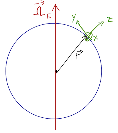
Last time, we set up the problem of studying the Coriolis deflection of a free-falling object on Earth's surface:
finding the equations of motion
\[ \begin{aligned} \ddot{x} = 2\Omega_E (\dot{y} \cos \theta - \dot{z} \sin \theta) \\ \ddot{y} = -2\Omega_E \dot{x} \cos \theta \\ \ddot{z} = -g + 2\Omega_E \dot{x} \sin \theta. \end{aligned} \]
To deal with these equations, we're going to use a technique known as perturbation theory.
Let me start by setting up the formal idea of a perturbative solution; this is an extremely common technique for solving physics problems, which you've certainly already seen used in a couple of particular cases (but probably not the general technique.)
Here is the setup: suppose that we have found an equation of motion of the form
\[ \begin{aligned} \ddot{r} = F(r, \epsilon) \end{aligned} \]
where \( \epsilon \) is a small, dimensionless parameter, and \( F \) is some totally arbitrary function. Of course, the obvious thing to do is expand the right-hand side in \( \epsilon \):
\[ \begin{aligned} \ddot{r} = F(r, 0) + \epsilon \frac{\partial F}{\partial \epsilon} + ... \end{aligned} \]
and then try to solve that equation. However, it's a common situation that this equation is still not easy to solve, and we can only really get the \( \epsilon = 0 \) version of the motion. Also, there are situations in which \( \epsilon \) is small but not too small, and we care about the discarded \( \epsilon^2 \) piece.
This brings us back to the idea of perturbation theory, which is to pre-emptively expand our solution in \( \epsilon \) as well, like this:
\[ \begin{aligned} r(t) = r^{(0)}(t) + \epsilon r^{(1)}(t) + \epsilon^2 r^{(2)}(t) + ... \end{aligned} \]
The piece of the solution \( r^{(n)} \) which is proportional to \( \epsilon^n \) is called the \( n \)-th order solution. (Note that I don't have the \( 1/2 \) in front of the \( \epsilon^2 \) term that would be there for a Taylor expansion. It would have been fine to include it, as long as we remember it when we put the pieces back together to get \( r(t) \)!)
Now we have a nice, systematic way to approach our solution. We start by simply solving the equation with \( \epsilon \) set to zero:
\[ \begin{aligned} \ddot{r}{}^{(0)} = F(r^{(0)}, 0) \end{aligned} \]
giving us the "zeroth-order" solution for \( r(t) \). Now we keep the first term in \( \epsilon \) on both sides:
\[ \begin{aligned} \ddot{r}{}^{(0)} + \epsilon \ddot{r}{}^{(1)} = F(r^{(0)}, 0) + \epsilon \frac{\partial F}{\partial \epsilon}(r^{(0)}, 0) \end{aligned} \]
Now, the beauty of this equation is that since \( \epsilon \) is just a parameter, it must be true for any value of \( \epsilon \), which means the \( \epsilon^1 \) pieces on both sides have to be equal:
\[ \begin{aligned} \epsilon \ddot{r}^{(1)} = \epsilon \frac{\partial F}{\partial \epsilon}(r^{(0)}). \end{aligned} \]
This is a much simpler differential equation for \( \ddot{r}^{(1)} \), especially because we already know what \( r^{(0)} \)(t) is on the right-hand side. Plus, it's very straightforward to keep going and find \( r^{(2)}(t) \) by keeping the \( \epsilon^2 \) pieces.
The key to using a perturbative solution is that you need a dimensionless small parameter to do the expansion in - never try to expand in something dimensionful in a physics problem, you'll probably just confuse yourself! The formal expressions will start to look a bit complicated if we keep going, so let's go back to our freefall problem.
Here are our equations of motion again:
\[ \begin{aligned} \ddot{x} = 2\Omega_E (\dot{y} \cos \theta - \dot{z} \sin \theta) \\ \ddot{y} = -2\Omega_E \dot{x} \cos \theta \\ \ddot{z} = -g + 2\Omega_E \dot{x} \sin \theta. \end{aligned} \]
We suspect that perturbation theory can be used here, because we know the effects of the Earth's rotation \( \Omega_E \) are often very small. But what is our small parameter? It's not simply \( \Omega_E \), because that would be dimensionful. Instead, I'll take the expansion parameter to be
\[ \begin{aligned} \epsilon = \Omega_E T, \end{aligned} \]
where \( T \) is the total time our object spends in free-fall. This makes physical sense: the longer our object is falling, the more important the fictitious forces will be, no matter how small \( \Omega_E \) is! (You might worry about the fact that we don't exactly know \( T \) yet, but it will end up cancelling out anyway in favor of the actual time \( t \). If you don't like \( T \) being the total time, just take it to be a fixed reference time that is definitely large compared to the freefall time, but not so large that \( \epsilon \) isn't tiny.)
We start at zeroth-order in \( \Omega_E T \), which basically just means we set \( \Omega_E = 0 \). Here we know the answer already: the only acceleration is \( \ddot{z} = -g \), and we find the usual free-fall motion. Setting initial conditions as starting from rest with \( x=y=0 \) and \( z=h \), we have
\[ \begin{aligned} x = x^{(0)}(t) = 0 \\ y = y^{(0)}(t) = 0 \\ z = z^{(0)}(t) = h - \frac{1}{2} gt^2, \end{aligned} \]
where the superscript \( (0) \) reminds us that these are zeroth-order; they don't depend on \( \Omega_E \) at all.
Now, on to first order. Notice what happens if we plug our series expansion into the \( x \) equation of motion above:
\[ \begin{aligned} \ddot{x} = 2\frac{\epsilon}{T} (\dot{y} \cos \theta - \dot{z} \sin \theta) \\ \ddot{x}^{(0)} + \epsilon \ddot{x}^{(1)} + ... = 2\frac{\epsilon}{T} \left[ (\dot{y}^{(0)} + \epsilon \dot{y}^{(1)} + ...) \cos \theta - (\dot{z}^{(0)} + \epsilon \dot{z}^{(1)} + ...) \sin \theta \right] \end{aligned} \]
Since we already know the zeroth-order solution, we just want to determine what \( \ddot{x}^{(1)} \) is here, which means we want all of the terms with one power of \( \epsilon \) on the right-hand side. Since there's already an \( \epsilon \) outside the brackets, and since \( y^{(0)}(t) = 0 \), we see there's only one:
\[ \begin{aligned} \epsilon \ddot{x}^{(1)} = -2\frac{\epsilon}{T} \dot{z}^{(0)} \sin \theta = 2\frac{\epsilon}{T} gt \sin \theta. \end{aligned} \]
This is the only equation in which \( \dot{z} \) appears, so we see that the other equations are unchanged to this order: formally,
\[ \begin{aligned} \ddot{y}^{(0)} + \epsilon \ddot{y}^{(1)} + ... = 0 + \mathcal{O}(\epsilon^2) \\ \ddot{z}^{(0)} + \epsilon \ddot{z}^{(1)} + ... = -g + \mathcal{O}(\epsilon^2) \end{aligned} \]
or reducing to equations just for the first-order pieces,
\[ \begin{aligned} \ddot{x}^{(1)} = 2g\frac{t}{T} \sin \theta \\ \ddot{y}^{(1)} = 0 \\ \ddot{z}^{(1)} = 0. \end{aligned} \]
Note that the \( 1/T \) in the equation for the \( x \)-acceleration fixes up the dimensions...
You can see what's happening here: at zeroth order, our object only moves in the \( z \)-direction, which means that the speed in the \( x \) and \( y \) directions is small. Motion in the \( z \)-direction gives a Coriolis deflection purely in the \( x \)-direction.
To get the complete solution, we have to put all the pieces back together: for example, we have
\[ \begin{aligned} \ddot{x}(t) \approx \ddot{x}^{(0)}(t) + \epsilon \ddot{x}^{(1)}(t) = 2\Omega_E g t \sin \theta \end{aligned} \]
Now we just integrate twice and impose the initial conditions to find our complete first-order solution:
\[ \begin{aligned} x(t) \approx \frac{1}{3} \Omega_E gt^3 \sin \theta, \\ y(t) \approx 0, \\ z(t) \approx h - \frac{1}{2} gt^2. \end{aligned} \]
Taylor stops at this point, but I say why not keep going to second order?
Clicker Question
What is the equation for the second-order perturbative acceleration \( \ddot{y}^{(2)} \)?
A. \( \ddot{y}^{(2)} = -2\dot{x}^{(0)}(t) \cos \theta -2\frac{\epsilon}{T} \dot{x}^{(1)} \cos \theta \)
B. \( \ddot{y}^{(2)} = -\frac{2}{T} \left(\dot{x}^{(0)}(t) + \epsilon \dot{x}^{(1)}\right) \cos \theta \)
C. \( \ddot{y}^{(2)} = -\frac{2}{T} \dot{x}^{(1)} \cos \theta \)
D. \( \ddot{y}^{(2)} = -\frac{2}{T} \dot{x}^{(2)} \cos \theta \)
E. \( \ddot{y}^{(2)} = -2\Omega_E \epsilon \dot{x}^{(1)} \cos \theta \)
Answer: C
(Note: this erroneously included an extra factor of \( \epsilon \) in class, so everyone gets full credit for it due to my mistake.)
This requires a little caution, but all we have to do is plug in the expansion
\[ \begin{aligned} y(t) = y^{(0)}(t) + \epsilon y^{(1)}(t) + \epsilon^2 y^{(2)}(t) + ... \end{aligned} \]
and similarly for \( \dot{x} \) on the right-hand side, and then isolate only the \( \epsilon^2 \) terms:
\[ \begin{aligned} ... + \epsilon^2 \ddot{y}^{(2)} = -2\frac{\epsilon}{T} \left( ... +\epsilon \dot{x}^{(1)} + ... \right) \cos \theta \end{aligned} \]
recovering answer C by matching the \( \epsilon^2 \) terms.
Applying this procedure to the other two equations, you should be able to arrive at the result
\[ \begin{aligned} \ddot{x}^{(2)} = \frac{2}{T} (\dot{y}^{(1)} \cos \theta - \dot{z}^{(1)} \sin \theta) \\ \ddot{y}^{(2)} = -\frac{2}{T} \dot{x}^{(1)} \cos \theta \\ \ddot{z}^{(2)} = \frac{2}{T} \dot{x}^{(1)} \sin \theta. \end{aligned} \]
This is easier to solve than it looks, since we know that both \( \dot{y}^{(1)} \) and \( \dot{z}^{(1)} \) are zero; plugging in \( \dot{x}^{(1)} = (gt^2/T) \sin \theta \) and integrating the other two equations gives us
\[ \begin{aligned} {y}^{(2)} = -\frac{1}{6} \frac{gt^4}{T^2} \cos \theta \sin \theta \\ {z}^{(2)} = \frac{1}{6} \frac{gt^4}{T^2} \sin^2 \theta \end{aligned} \]
so for the full second-order solution, we add each of these terms multiplied by \( \epsilon^2 = (\Omega_E T)^2 \):
\[ \begin{aligned} x(t) = \frac{1}{3} \Omega_E gt^3 \sin \theta + \mathcal{O}(\epsilon^3) \\ y(t) = -\frac{1}{6} \Omega_E^2 gt^4 \cos \theta \sin \theta + \mathcal{O}(\epsilon^3) \\ z(t) = h - \frac{1}{2} gt^2 + \frac{1}{6} \Omega_E^2 gt^4 \sin^2 \theta + \mathcal{O}(\epsilon^3) \end{aligned} \]
Hopefully you can appreciate that this is a really nice trick for solving differential equations when a small parameter is involved! Everything we've done is totally rigorous; you will find the same answer if you solve the system exactly (Mathematica can do this, e.g.) and then series expand the solutions that you find.
You should be careful with boundary conditions when applying this technique, since the total solution has to satisfy those, not just the individual pieces. (Typically, as happened here, the zeroth-order solutions will handle any nontrivial boundary conditions, and then the higher-order terms all simply vanish at the boundaries.)
We should emphasize that, justifying our series expansion treatment, this is a small but not compeltely negligible!) effect. The book gives the example of a 100m mine shaft at the equator, which gives a horizontal deflection at first order in \( \Omega_E \) of about 2 cm. The (zeroth-order) time in freefall is \( \sqrt{2h/g} = 4.5 \) seconds, so \( \epsilon = \Omega_E T \approx 3 \times 10^{-4} \) - small indeed, so we trust our expansion! Indeed, if we look at 45 degrees latitude instead, then the (first-order) x-deflection is 1.6 cm, but the predicted (second-order) y-deflection is only 1.8 micrometers.
One last nice example of motion on the rotating Earth is the Foucault pendulum; I won't cover this in lecture, but Taylor does it in detail in chapter 9.9. If you haven't seen one in person before, check out the operating Foucault pendulum in the base of the Gamow tower right here in our own physics building (you can see it from the outside.)