Matrices are everywhere in physics, much like vectors. In fact, matrices show up so often exactly because vectors are so important in the description of physical laws. The product of a matrix with a vector is another vector,
\[ \begin{aligned} \vec{v'} = \mathbf{O} \vec{v}, \end{aligned} \]
so you can think of a matrix as an operator, acting on the space of vectors \( v \): it's a machine that takes a vector and input and gives you another one as output.
For \( \vec{v} \) and \( \vec{v'} \) in an \( n \)-dimensional vector space (for our purposes, usually the familiar three-dimensional space), the matrix \( \mathbf{O} \) is an \( n \times n \) square matrix.
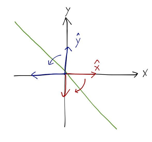
Simple example to see how this works! Consider a plane with a mirror across it at a \( 45^\circ \) angle, i.e. sitting on the line \( y=-x \). If we draw a vector in the top right, there will be a mirror image in the bottom left. The mirror image is a transformed version of the original vector.
What does the mirror image look like? The image vector should have the same length and make the same angle with the mirror. If we look at the unit vectors, then we see that
\[ \begin{aligned} \hat{x} \rightarrow -\hat{y}, \\ \hat{y} \rightarrow -\hat{x}. \end{aligned} \]
What about an arbitrary vector \( \vec{v} \)? Well, it turns out that we're already done, because \( \mathbf{M} \) is a special type of operator called a linear operator. Linear operators satisfy the following two conditions:
- Applying the operator to a vector rescaled by a constant, \( c\vec{v} \), gives us back the operator applied to the original vector, and then rescaled:
\[ \begin{aligned} \mathbf{O} (c \vec{v}) = c \left(\mathbf{O} \vec{v} \right); \end{aligned} \]
- Applying the operator to a sum of two vectors \( \vec{v_1} + \vec{v_2} \) is equivalent to applying it to both vectors and then adding them:
\[ \begin{aligned} \mathbf{O} (\vec{v_1} + \vec{v_2}) = \mathbf{O} \vec{v_1} + \mathbf{O} \vec{v_2}. \end{aligned} \]
In fact, any operator which is described by a matrix automatically has these properties. (Non-linear operators do exist, but are rare, and we certainly won't see any this semester.)
Thanks to linearity, we thus know how \( \mathbf{M} \) acts on any vector: it takes \( (v_x, v_y) \) into \( (-v_y, -v_x) \). We can thus write the operation of reflecting about the line \( y=-x \) as,
\[ \begin{aligned} \mathbf{M} = \left( \begin{array}{cc} 0&-1\\-1&0\end{array} \right). \end{aligned} \]
For example, the mirror image of the vector \( (1,2) \) is
\[ \begin{aligned} \left( \begin{array}{cc} 0&-1\\-1&0\end{array} \right) \left( \begin{array}{c} 1\\2 \end{array} \right) = \left( \begin{array}{c} -2\\-1\end{array} \right) \end{aligned} \]
Matrices show up very often in physics, especially as operators. Another example is rotation: rotating a vector about the origin by an angle \( \alpha \) can be written as a rotation matrix. We can easily find the matrix form once again by looking at what happens to the unit vectors:
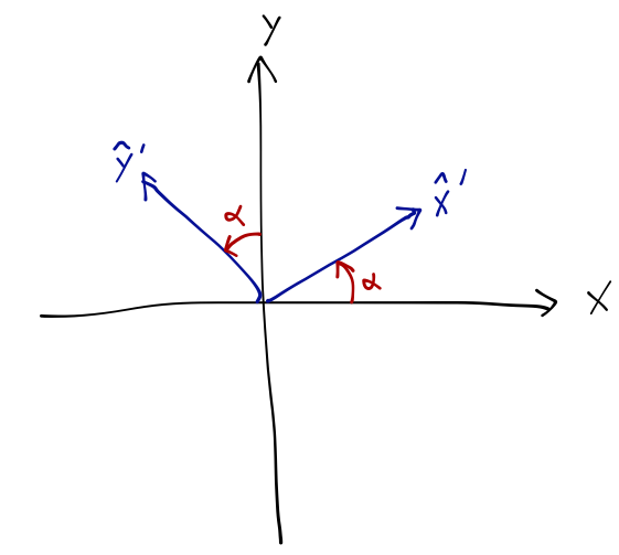
\[ \begin{aligned} \hat{x} \rightarrow \cos \alpha \hat{x} + \sin \alpha \hat{y} \\ \hat{y} \rightarrow -\sin \alpha \hat{x} + \cos \alpha \hat{y} \end{aligned} \]
so we can immediately write down
\[ \begin{aligned} \mathbf{R}(\alpha) = \left( \begin{array}{cc} \cos \alpha&\sin \alpha\\ -\sin \alpha & \cos \alpha \end{array} \right). \end{aligned} \]
Other examples involve more complicated relations, and can change units for example. For example, we know that for rotation of an object about a single axis, its angular momentum \( L \) is
\[ \begin{aligned} L = I \omega, \end{aligned} \]
where \( I \) is the moment of inertia about that axis, and \( \omega \) is the angular velocity. But what if we can't just work with a single fixed axis? If you throw a book in the air, it will tumble in a complicated way even though no forces are acting on it in mid-air; since \( \vec{L} \) is fixed, but apparently \( \vec{\omega} \) is not, the only explanation is that \( I \) is really an operator, the inertia operator, and the more general equation is
\[ \begin{aligned} \vec{L} = \mathbf{I} \vec{\omega}. \end{aligned} \]
We will explore this equation in detail when we come to the rotation of rigid bodies shortly.
Some matrix basics
The components of a matrix are written out with respect to a basis, which is just a set of unit vectors which can be combined to reach any point in the \( n \)-dimensional space. Remember that if you change coordinates, any matrix quantities change too!
I will drop the arrow notation for now, since we're going to be writing a lot of matrices down and it shouldn't be confusing in context. In linear algebra, matrices are usually denoted by capital letters \( A, B, C, ... \), while vectors and scalars are lower-case letters.
Some basic rules of (square) matrix manipulation, which I'll go through fast because you should know them:
- Matrix equality
Two matrices are equal if and only if they have the same dimensions, and every component is equal. So
\[ \begin{aligned} \left( \begin{array}{cc} x&r\\ y&s \end{array} \right) = \left( \begin{array}{cc} 2&1 \\ 3&-5\end{array} \right) \end{aligned} \]
implies the four equations
\[ \begin{aligned} x = 2, y = 3, r = 1, s = -5. \end{aligned} \]
This is foreshadowing the other use of matrices which we will encounter, which is to compactly write a system of equations as a single matrix equation. For example, if we have two masses connected by springs to each other and to a wall on either side, the equations of motion are
\[ \begin{aligned} m\ddot{x_1} = -(k_1 + k_2) x_1 + k_2 x_2 \\ m\ddot{x_2} = k_2 x_1 - (k_2 + k_3) x_2 \end{aligned} \]
which can be written in in the much more compact form
\[ \begin{aligned} m \left( \begin{array}{c} \ddot{x_1} \\ \ddot{x_2} \end{array} \right) = - \left( \begin{array}{cc} k_1 + k_2 & -k_2 \\ -k_2 & k_2 + k_3 \end{array} \right) \left( \begin{array}{c} x_1 \\ x_2 \end{array} \right) \end{aligned} \]
or simply \( \ddot{\vec{x}} = -\frac{1}{m} \mathbf{K} \vec{x} \).
The application of matrix algebra will allow us to quickly and generally find solutions to these systems.
- Index notation
You know that we can write the components of a vector in terms of an index, which iterates over the \( n \) coordinates in our vector space: for a Cartesian vector, we write \( v_i \), where \( i = 1,2,3 \) (or \( x,y,z \).)
We can write the components of a matrix out in exactly the same way, but for a matrix we need a pair of indices: one to specify the row, one for the column. By convention, the first index is the row index.
\[ \begin{aligned} A = \left( \begin{array}{ccc} 2&1&6 \\ 3&-5&0 \\ 1&-4&9 \end{array} \right) \Rightarrow A_{21} = 3, A_{13} = 6, A_{33} = 9, ... \end{aligned} \]
- Multiplying by a number
To multiply a matrix by a number \( c \), we just multiply every component by \( c \).
\[ \begin{aligned} 2 \left( \begin{array}{cc} 2&1 \\ 3&-5\end{array} \right) = \left( \begin{array}{cc} 4&2 \\ 6&-10\end{array} \right) \end{aligned} \]
- Addition of matrices
Matrices add (or subtract) component by component, just like vectors do.
\[ \begin{aligned} \left( \begin{array}{cc} 2&1 \\ 3&-5\end{array} \right) + \left( \begin{array}{cc} 1&0 \\ -2&3\end{array} \right) = \left( \begin{array}{cc} 3&1 \\ 1&-2\end{array} \right). \end{aligned} \]
- Matrix-vector multiplication
When a vector is to the right of a matrix, we write it as a column and multiply by the rows of the matrix,
\[ \begin{aligned} \left( \begin{array}{cc} 2&1 \\ 3&-5\end{array} \right) \left( \begin{array}{c} 2\\ -1\end{array} \right) = \left( \begin{array}{c} 2(2) + 1(-1) \\ 2(3) + (-1)(-5) \end{array} \right) = \left( \begin{array}{c} 3 \\ 11 \end{array} \right). \end{aligned} \]
On the other hand, a vector to the left of a matrix is written as a row and multiplies the columns:
\[ \begin{aligned} \left(2\ \ \ -1\right) \left( \begin{array}{cc} 2&1 \\ 3&-5\end{array} \right) = \left(2(2) + (-1)(3)\ \ \ 2(1) + (-1)(-5) \right) \\ = \left(1\ \ \ 7\right). \end{aligned} \]
Notice that the answer depends on which side the vector is on! In index notation, we can expand out: if \( \vec{w} = A\vec{v} \), then
\[ \begin{aligned} w_i = \sum_j A_{ij} v_j \end{aligned} \]
while for left multiplication \( \vec{w}'' = \vec{v} A \),
\[ \begin{aligned} w_i' = \sum_j v_j A_{ji}. \end{aligned} \]
- Matrix-matrix multiplication
The rule for multiplying two matrices together is a generalization of the above: we multiply the columns of the right-hand matrix by the rows of the left-hand matrix, one by one. If \( C = AB \), then the element \( C_{ij} \) in row \( i \), column \( j \) of the product matrix \( C \) is given by row \( i \) of matrix \( A \), times column \( j \) of matrix \( B \), i.e.
\[ \begin{aligned} C_{ij} = \sum_{k} A_{ik} B_{kj}. \end{aligned} \]
If you take the columns of \( B \) from left to right and multiply by rows of \( A \), you will build up \( C \) column by column, starting at the left.
\[ \begin{aligned} \left( \begin{array}{cc} 2&1 \\ 3&-5\end{array} \right) \left( \begin{array}{cc} 3&-1 \\ -4&2\end{array} \right) = \left( \begin{array}{cc} 2&0 \\ 29&-13\end{array} \right). \end{aligned} \]
Once again, order of operations matters: \( AB \neq BA \)! In fact, we define an object called the commutator as the difference,
\[ \begin{aligned} [A,B] \equiv AB - BA. \end{aligned} \]
The opposite of this, which you'll run into less frequently, is the anti-commutator
\[ \begin{aligned} \{A, B\} \equiv AB + BA. \end{aligned} \]
We can now also define a power of a matrix: \( A^n \) is just the matrix \( A \) multiplied by itself \( n \) times.
\[ \begin{aligned} \left( \begin{array}{cc} 2&1 \\ 3&-5\end{array} \right)^2 = \left( \begin{array}{cc} 2&1 \\ 3&-5\end{array} \right) \left( \begin{array}{cc} 2&1 \\ 3&-5\end{array} \right) = \left( \begin{array}{cc} 7&-3 \\ -9&28\end{array} \right) \end{aligned} \]
- Identity and zero matrices
The identity matrix, \( 1 \), has all \( 1 \)'s on the diagonal, and \( 0 \) elsewhere; the zero matrix, \( 0 \), has all zero entires. You'll sometimes see the identity in \( n \) dimensions written as \( 1_n \).
\[ \begin{aligned} 1_3 = \left( \begin{array}{ccc} 1&0&0\\ 0&1&0\\ 0&0&1\end{array} \right) \end{aligned} \]
Adding the zero matrix, or multiplying by the identity matrix, just gives you back the same matrix.
\[ \begin{aligned} A + 0 = A \\ 1A = A1 = A \end{aligned} \]
- Trace and determinant
Two operations which are special to matrices are the trace and the determinant. The trace of a matrix is just the sum of all the diagonal elements:
\[ \begin{aligned} \textrm{tr}(A) = \sum_i A_{ii}. \end{aligned} \]
An example:
\[ \begin{aligned} \textrm{tr} \left( \begin{array}{cc} 2&1 \\ 3&-5\end{array} \right) = 2-5 = -3. \end{aligned} \]
The trace is distributive over sums of matrices, i.e.
\[ \begin{aligned} \textrm{tr} (A+B) = \textrm{tr} (A) + \textrm{tr} (B), \end{aligned} \]
Trace is also invariant under cyclic permutation, i.e.
\[ \begin{aligned} \textrm{tr} (ABC) = \textrm{tr} (BCA) = \textrm{tr} (CAB). \end{aligned} \]
This is easy to see if you write everthing out in terms of indices, for instance
\[ \begin{aligned} \textrm{tr} (AB) = \sum_i \sum_j A_{ij} B_{ji} = \sum_i \sum_j B_{ji} A_{ij}. \end{aligned} \]
The determinant is a very useful function of a matrix, but is a little harder to define. For any two-by-two matrix, the determinant (which is written with straight lines) is equal to
\[ \begin{aligned} \det \left( \begin{array}{cc} a&b\\c&d \end{array} \right) = \left| \begin{array}{cc} a&b\\c&d \end{array} \right| = ad - bc. \end{aligned} \]
There are a few ways to calculate determinants of larger matrices, but the easiest to remember is the technique of expansion in minors. The algorithm is as follows:
- Pick any single row or column of the matrix - usually the top row, but you will get the same answer no matter what!
- For each element of that row or column, the corresponding minor is equal to the determinant of a smaller matrix, namely the original matrix with the row and column of our chosen element removed.
- The determinant is equal to the sum of elements times minors, including an additional minus sign whenever the sum of row and column indices of the element are odd. (This last requirement means that we add or subtract element times minor according to a checkerboard pattern, e.g. for a 4x4 matrix:)
\[ \begin{aligned} \left| \begin{array}{cccc} +&-&+&- \\ -&+&-&+ \\ +&-&+&- \\ -&+&-&+ \end{array} \right|. \end{aligned} \]
Let's do an example!
\[ \begin{aligned} \left| \begin{array}{ccc} -2&1&6 \\ 3&-5&0 \\ 1&-4&9 \end{array} \right| = -2 \left| \begin{array}{cc} -5&0\\ -4&9\end{array} \right| - 1 \left| \begin{array}{cc} 3&0\\ 1&9\end{array} \right| + 6 \left| \begin{array}{cc} 3&-5\\ 1&-4\end{array} \right| \\ = -2 (-45 - 0) -1 (27 - 0) + 6 (-12+5) = 21. \end{aligned} \]
This is easy to do by hand for 3x3 matrices, and reasonable for 4x4; employing something like Mathematica is probably a better option if you run into larger matrices than that.
One very useful fact: the determinant is distributive over products of matrices,
\[ \begin{aligned} \det (AB) = \det A \det B = \det(BA). \end{aligned} \]
- Matrix inverse
The inverse of a matrix \( A \) is the matrix which when multiplied by \( A \) gives the identity matrix,
\[ \begin{aligned} A A^{-1} = A^{-1} A = \mathbf{1}. \end{aligned} \]
The inverse of a product of matrices is equal to the product of the inverses, but in reverse order:
\[ \begin{aligned} (ABCD)^{-1} = D^{-1} C^{-1} B^{-1} A^{-1}. \end{aligned} \]
You can see this easily by applying those four matrices on the left or right in turn to the product \( ABCD \).
Not every matrix has an inverse! If \( A^{-1} \) does exist, then \( A \) is said to be invertible; if there is no \( A^{-1} \), then \( A \) is said to be singular. The determinant provides a very useful test for singular matrices! We can prove this quickly: take the determinant of both sides of the definition above,
\[ \begin{aligned} \det(A A^{-1}) = \det(\mathbf{1}) \\ \det(A) \det(A^{-1}) = 1 \end{aligned} \]
which tells us that
\[ \begin{aligned} \det(A^{-1}) = \frac{1}{\det(A)}. \end{aligned} \]
But this relation is only possible if \( \det(A) \neq 0 \)! So any matrix with \( \det(A) = 0 \) must be singular. This doesn't prove that every square matrix with non-zero determinant is invertible, of course, but that happens to be true as well.
- Transpose and orthogonality
The transpose of a matrix (denoted \( A^T \)) is obtained by swapping the rows and columns, or equivalently, reflecting all of the entries across the diagonal.
\[ \begin{aligned} \left( \begin{array}{cc} 2&1 \\ 3&-5\end{array} \right)^T = \left( \begin{array}{cc} 2&3 \\ 1&-5\end{array} \right). \end{aligned} \]
Like the inverse, the transpose acts on a product of matrices by giving the same product in reverse order,
\[ \begin{aligned} (AB)^T = B^T A^T. \end{aligned} \]
If a matrix is equal to its own transpose, \( A = A^T \), then it is said to be a symmetric matrix. On the other hand, if the transpose of a matrix is also its inverse,
\[ \begin{aligned} A^T = A^{-1}, \end{aligned} \]
then it is said to be an orthogonal matrix. Orthogonal matrices have a number of special properties, and they occur often in physics applications. In fact, you can check that the reflection matrix and the rotation matrix we considered above are both orthogonal matrices.
Orthogonal matrices have a number of special properties, but one of the most important is that they are length-preserving: an operator described by an orthogonal matrix doesn't change the length of any vector.
Eigenvalues and eigenvectors
Let's go back to the mirror operation from above. Are there any vectors which the reflection operation leaves unchanged?
Clicker Question
Which two-dimensional vectors are mapped into themselves by mirror reflection (up to a constant)?
A. \( \hat{x} \) and \( \hat{y} \)
B. \( \hat{x} + \hat{y} \) and \( \hat{x} - \hat{y} \)
C. Just \( \hat{x} + \hat{y} \)
D. Just \( \hat{x} - \hat{y} \)
E. Any vector is mapped to itself times a constant.
Answer: B
We can start by ruling out E, because we have the two unit-vector examples in front of us: for example, \( \hat{y} \) becomes \( -\hat{x} \), which is not a constant times the original! Similarly A doesn't work; those vectors are mapped into each other (times -1), but not into themselves.
That leaves the two vectors given in the middle three choices. \( \hat{x} - \hat{y} \) is the vector that points along the mirror, i.e. along the line \( y=-x \); it should be obvious that reflection does nothing to these vectors, so they're just mapped to themselves. We can see this from the matrix math:
\[ \begin{aligned} \left( \begin{array}{cc} 0&-1 \\ -1&0\end{array} \right) \left( \begin{array}{c} 1 \\ -1 \end{array} \right) = \left( \begin{array}{c}1 \\ -1 \end{array} \right) \end{aligned} \]
or in other words, \( M\vec{v}_1 = \vec{v}_1 \).
What about \( \hat{x} + \hat{y} \)? If we try the matrix operation, then we find
\[ \begin{aligned} \left( \begin{array}{cc} 0&-1 \\ -1&0\end{array} \right) \left( \begin{array}{c} 1 \\ 1 \end{array} \right) = \left( \begin{array}{c}-1 \\ -1 \end{array} \right). \end{aligned} \]
So the reflection leaves this vector pointing in the same direction, but multiplied by a constant, -1: \( M \vec{v}_2 = -\vec{v}_2 \). Thus, both vectors are mapped into themselves times a constant.
You may already recognize these as the eigenvectors of the mirror operation - we'll come back to eigenvalues and eigenvectors next time.