Last time, after some general review of matrix math and notation, we ended on a clicker question about vectors and mirror reflection:
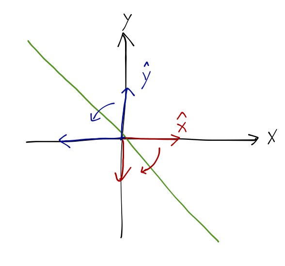
The mirror reflection operation can be represented as the matrix
\[ \begin{aligned} \mathbf{M} = \left( \begin{array}{cc} 0&-1\\-1&0\end{array} \right), \end{aligned} \]
In the clicker question, we identified the two vectors \( \vec{v}_1 = \hat{x} - \hat{y} \) and \( \vec{v}_2 = \hat{x} + \hat{y} \) which are mapped to themselves times a constant, i.e. they represent solutions to the equation
\[ \begin{aligned} M \vec{v_i} = \lambda_i \vec{v_i}. \end{aligned} \]
The vectors solving this equation, the ones which the matrix doesn't change the direction of, are called eigenvectors of \( M \). The rescaling factor \( \lambda_i \) associated with each eigenvector is called its eigenvalue. So the reflection matrix has two eigenvalues: \( \lambda_1 = +1, \lambda_2 = -1 \).
What is the point of finding the directions which our reflection operation leaves unchanged? Notice that for any vector in the space, we could have split it into components along the two vectors \( \vec{v}_1, \vec{v}_2 \). The reflection operation is then particularly simple: we do nothing to the \( \vec{v}_1 \) component, and multiply the \( \vec{v}_2 \) component by \( -1 \). In other words, in a coordinate system defined by the eigenvectors, the matrix is diagonal, and its entries are the associated eigenvalues.
Often in physics, you have seen that picking a "clever" set of coordinates for a particular problem allows you to easily solve for the motion; for example, on the homework you solved for the motion of two masses connected by a spring, and found that changing coordinates to the center of mass and the separation distance of the two masses made the problem much simpler. The great power of the eigenvector and eigenvalue approach is that it doesn't require a clever guess; we will now have an algorithm to decide what the physically important directions are, and to tell us how to change coordinates accordingly!
For the reflection matrix, it was easy to see what the eigenvectors were. But how do we solve for them more generally? Remember that we're solving the equation
\[ \begin{aligned} A \vec{v} = \lambda \vec{v} \end{aligned} \]
for some matrix \( A \). We can rewrite the right-hand side also as a matrix-vector product by using the identity: \( \lambda \vec{v} = \lambda I \vec{v} \). Then subtracting, we have
\[ \begin{aligned} (A - \lambda I) \vec{v} = 0. \end{aligned} \]
This equation is always true if \( \vec{v} = 0 \), but this is the trivial solution - we're interested in solutions involving non-zero vectors. It is a fundamental result of linear algebra (which I won't prove) that the equation \( M \vec{v} = 0 \) has non-trivial solutions if, and only if, \( \det(M) = 0 \). This means that if \( \lambda \) is an eigenvalue of \( A \), then it must satisfy the equation
\[ \begin{aligned} \det (A - \lambda I) = 0. \end{aligned} \]
If \( A \) is an \( nxn \) matrix, this equation will be an \( n \)-th order polynomial in \( \lambda \), known as the characteristic polynomial; its solutions are the eigenvalues of \( A \).
Let's do an example! Suppose we're given the matrix
\[ \begin{aligned} A = \left( \begin{array}{cc} 5&-2 \\ -2&2 \end{array} \right). \end{aligned} \]
The characteristic polynomial is then
\[ \begin{aligned} |A - \lambda I| = \left| \begin{array}{cc} 5-\lambda&-2 \\ -2&2-\lambda \end{array} \right| \\ = (5-\lambda) (2-\lambda) - 4. \end{aligned} \]
Solving for the roots:
\[ \begin{aligned} (5-\lambda) (2-\lambda) - 4 = 0 \\ \lambda^2 - 7 \lambda + 10 - 4 = 0 \\ \lambda = \frac{1}{2} (7 \pm \sqrt{49 - 24}) \\ = \frac{1}{2} (7 \pm 5) \\ = 1, 6. \end{aligned} \]
Once we have the eigenvalues, it's straightforward to find the eigenvectors: just plug in to the equation \( A \vec{v} = \lambda \vec{v} \) and solve. Let's try it! First, \( \lambda_1 = 1 \):
\[ \begin{aligned} \left( \begin{array}{cc} 5&-2 \\ -2&2\end{array} \right) \left( \begin{array}{c} x_1 \\ y_1 \end{array} \right) = 1 \left( \begin{array}{c} x_1 \\ y_1 \end{array} \right) \\ \left( \begin{array}{c} 5x_1- 2y_1 \\ -2x_1 + 2y_1 \end{array} \right) = \left( \begin{array}{c} x_1 \\ y_1 \end{array} \right) \\ \left( \begin{array}{c} 4x_1 - 2y_1 \\ -2x_1 + y_1 \end{array} \right) = \left( \begin{array}{c} 0 \\ 0 \end{array} \right) \end{aligned} \]
Both of these equations are satisfied so long as \( 2x_1 = y_1 \). This ambiguity shouldn't surprise you; since the condition on an eigenvector is just that its direction doesn't change when the matrix is applied, the length of the vector is arbitrary. It is usually convenient to normalize the eigenvectors as unit vectors, so let's do that: in addition to \( 2x_1 = y_1 \), we have \( x_1^2 + y_1^2 = 5x_1^2 = 1 \), so the unit eigenvector is
\[ \begin{aligned} \hat{v_1} = \frac{1}{\sqrt{5}} \left( \begin{array}{c} 1 \\ 2 \end{array} \right). \end{aligned} \]
We can do the same exercise for the other eigenvalue \( \lambda_2 = 6 \), and we will find
\[ \begin{aligned} \hat{v_2} = \frac{1}{\sqrt{5}} \left( \begin{array}{c} -2 \\ 1 \end{array} \right). \end{aligned} \]
Notice that our eigenvectors are orthogonal to each other; that is, \( \hat{v_1} \cdot \hat{v_2} = 0 \). This is not a coincidence; it is a consequence of the fact that our original matrix \( A \) was symmetric. Any real, symmetric matrix has only real (non-complex) eigenvalues, and orthogonal eigenvectors. (You can use this as a trick to find the last eigenvector, if you've already found the first \( n-1 \) for an \( n \times n \) matrix.)
We haven't talked very much about changes of basis and matrices, but I will just state without proof that for a symmetric matrix, as long as we have \( n \) independent eigenvectors, then we can always change coordinates to use the unit eigenvectors as our basis vectors, and in that basis the matrix becomes diagonal:
\[ \begin{aligned} A \rightarrow \left( \begin{array}{cccc} \lambda_1&&&\\ &\lambda_2&& \\ &&...& \\ &&&\lambda_n \end{array} \right) \end{aligned} \]
Note that the order of the eigenvalues matters, and corresponds to the order of the eigenvectors.
Some facts satisfied by the determinant and trace: the determinant of a matrix is equal to the product of its eigenvalues, and the trace is equal to the sum.
\[ \begin{aligned} \det A = \lambda_1 \lambda_2 ... \lambda_n \\ \textrm{tr} A = \lambda_1 + \lambda_2 + ... + \lambda_n. \end{aligned} \]
We haven't talked very much about changes of basis, but these both follow from the fact that changing to the basis specified by the eigenvectors is a "similarity transformation", which leaves the eigenvalues unchanged. It's easy to see that in the basis of the eigenvectors, where \( A \) becomes diagonal, that the trace and determinant are exactly given by these formulas.
There are two special cases that can happen as we go through this procedure. The first is the occurrence of degenerate eigenvalues, that is, the same eigenvalue appearing more than once as a solution to the characteristic polynomial. For example, the matrix
\[ \begin{aligned} \left(\begin{array}{ccc} 0&1&1\\ 1&0&1\\ 1&1&0 \end{array} \right) \end{aligned} \]
has characteristic polynomial
\[ \begin{aligned} -\lambda^3 + 2 + 3\lambda = -(\lambda - 2) (\lambda+1)^2 \end{aligned} \]
so there is a pair of \( -1 \) eigenvalues, and a single \( 2 \). If we try to solve for the \( -1 \) eigenvector, we will find the equation
\[ \begin{aligned} \left(\begin{array}{ccc} 1&1&1\\ 1&1&1\\ 1&1&1 \end{array} \right) \left( \begin{array}{c} x \\ y \\ z \end{array} \right) = 0. \end{aligned} \]
This is one equation for three unknowns; the equation defines a plane in our three-dimensional space. So the eigenspace associated with the paired eigenvalue has dimension 2. We can still construct a set of orthogonal eigenvectors, but we have freedom to choose any pair that lies in the plane defined by the equation \( x+y+z = 0 \).
Angular momentum of rigid objects
In most of our discussion of mechanics this semester, we've been treating everything like a point particle. Point particles can only translate - move around in space - and unconstrained, have \( 3 \) degrees of freedom, i.e. we need 3 numbers to uniquely specify each particle's location.
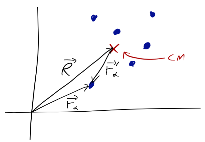
Now we'll extend our attention to rigid bodies; collections of many particles held together in a fixed shape (ignoring bending, stretching, etc.) For a system of \( N \) particles (label: \( \alpha = 1, ..., N \)), we know that we can treat collective motion as if all mass and forces were concentrated at the center of mass,
\[ \begin{aligned} \vec{F}_{\textrm{ext}} = M \ddot{\vec{R}}, \end{aligned} \]
where \(M = \sum_{\alpha=1}^{N} m_\alpha\), and the CM position is
\[ \begin{aligned} \vec{R} = \frac{1}{M} \sum_{\alpha=1}^{N} m_\alpha \vec{r}_\alpha. \end{aligned} \]
In principle, we need \( 3N \) different coordinates to describe such a collection of particles - and \( N \) is incredibly large for macroscopic objects, if we treat them as collections of atoms! However, the requirement that we have a rigid body provides almost as many constraints. There are only two kinds of motion that a rigid body can undergo: translation of the center of mass, and rotation about the center of mass. (This is hopefully an intuitive statement, but we'll demonstrate it shortly!)
Although I'm going to derive a lot of results using sums like this, keep in mind that an everyday object is made up of such an enormous number of individual atoms that we can, to good approximation, just treat the object as a continuous distribution of matter. In that case, we can write integrals instead of sums,
\[ \begin{aligned} \vec{R} = \frac{1}{M} \int \vec{r}\ dm. \end{aligned} \]
So again, although we'll derive a lot of facts using sums, in practice we'll mostly be working with integrals in this subject.
There was one example of a system we didn't treat as simply a point particle with Lagrangian mechanics: a rolling object.
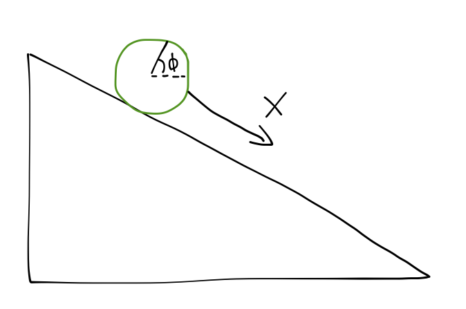
As we saw, the kinetic energy of the rolling disk has two components:
\[ \begin{aligned} T = \frac{1}{2} m \dot{x}^2 + \frac{1}{2} I \dot{\phi}^2. \end{aligned} \]
The first term is the usual translational kinetic energy, while the second term is the kinetic energy associated with the rotation of the disk. Because the disk is an extended object, it is able to store energy internally, even if it isn't moving in space. For example, if we mounted the disk on a rod and just spun it about its axis without letting it go anywhere (this is a "flywheel"), it still has kinetic energy - energy associated with its motion.
Let's generalize beyond the disk. For any system of \( N \) particles, the total kinetic energy is just the sum of the individual particle kinetic energies,
\[ \begin{aligned} T = \sum_{\alpha = 1}^N \frac{1}{2} m_\alpha \dot{\vec{r}}_\alpha^2. \end{aligned} \]
We can split each position vector \( \vec{r}\alpha \) into two components: the CM position vector \( \vec{R} \), and the position of the particle relative to the CM, \( \vec{r}'\alpha \).
\[ \begin{aligned} \vec{r}_\alpha = \vec{R} + \vec{r}'_\alpha. \end{aligned} \]
For the kinetic energy, then, we have
\[ \begin{aligned} T = \frac{1}{2} \sum_\alpha m_\alpha (\dot{\vec{R}}^2 + \dot{\vec{r}}'_\alpha{}^2 + 2 \dot{\vec{R}} \cdot \dot{\vec{r}}'_\alpha). \end{aligned} \]
We can rewrite the last term as
\[ \begin{aligned} T = (...) + \dot{\vec{R}} \sum_\alpha m_\alpha \dot{\vec{r}}'_\alpha \\ = \dot{\vec{R}} \frac{d}{dt} \left( \sum_\alpha m_\alpha \vec{r}'_\alpha \right). \end{aligned} \]
This sum looks exactly like the definition of the CM, except now it's in coordinates relative to the CM itself! So it's just equal to zero. We can show this mathematically: going back to the definition of the CM, notice that
\[ \begin{aligned} M \vec{R} = \sum_\alpha m_\alpha \vec{r}_\alpha \\ \Rightarrow 0 = \sum_\alpha (m_\alpha \vec{r}_\alpha - M \vec{R}) \\ = \sum_\alpha (m_\alpha (\vec{R} + \vec{r}'_\alpha) - M\vec{R}) \\ = \sum_\alpha m_\alpha \vec{r}'_\alpha \end{aligned} \]
since \( \sum_\alpha m_\alpha = M \). So crossing the last term out, we have for the total kinetic energy
\[ \begin{aligned} T = \frac{1}{2} M \dot{\vec{R}}^2 + \frac{1}{2} \sum_\alpha m_\alpha \dot{\vec{r}}'_\alpha{}^2 \\ = T_{CM} + T_{\textrm{rel}}. \end{aligned} \]
For any collection of particles, total \( T \) splits into \( T \) associated with motion of the center of mass, plus \( T \) relative to center of mass.
If only central, conservative forces are involved, \( U \) can be divided up similarly,
\[ \begin{aligned} U = U_{ext} + U_{int} = U_{ext} + \sum_\alpha \sum_\beta U_{\alpha \beta} (|\vec{r}_\alpha - \vec{r}_\beta|). \end{aligned} \]
(Non-central internal forces can mess with total angular momentum, a complication we want to avoid for now.)
So, extended objects can store energy internally, and it can be treated more or less separately from CM motion (which acts like a point particle.) A flywheel stores kinetic energy internally; a spring stores potential energy internally. (This is mechanics and not E&M, but of course there's a close analogy here to a battery, which stores electric potential energy internally.)
Rotation of rigid bodies
The above derivation was actually totally general, but from now on we'll restrict our attention to rigid bodies. A rigid body is a collection of particles which have fixed positions relative to each other. Any solid is a rigid body, ignoring deformation (effects like stretching and bending.)
Fixed relative distance means the internal potential energy becomes an (ignorable) constant:
\[ \begin{aligned} U_{\textrm{rigid}} = U_{ext}. \end{aligned} \]
Rigid bodies can still store internal kinetic energy through rotation, which is the only motion which preserves all inter-particle distances.
\[ \begin{aligned} T = T_{CM} + T_{\textrm{rot}}. \end{aligned} \]
Since we're interested in rotation, we should look at the angular momentum of our collection of particles. Recall that for a point particle,
\[ \begin{aligned} \vec{L} = \vec{r} \times \vec{p} = m \vec{r} \times \dot{\vec{r}}. \end{aligned} \]
I'll skip the derivation, but in fact \( \vec{L} \) divides up just like energy does, between the CM and motion relative to the CM:
\[ \begin{aligned} \vec{L} = M \vec{R} \times \dot{\vec{R}} + \sum_\alpha m_\alpha \vec{r}'_\alpha \times \dot{\vec{r}}'_\alpha \\ = \vec{L}_{CM} + \vec{L}_{\textrm{rel}}. \end{aligned} \]
(Derivation is in 10.1 of Taylor; it's very similar to our kinetic energy derivation.)
Another reminder: the angular equivalent of force is the torque, for a point particle
\[ \begin{aligned} \vec{\Gamma} = \vec{r} \times \vec{F}. \end{aligned} \]
(Some people prefer \( \vec{\tau} \) for torque, but I'll follow Taylor and use \( \vec{\Gamma} \).) Torque and angular momentum are related just like force and linear momentum, i.e.
\[ \begin{aligned} \vec{\Gamma} = \dot{\vec{L}}. \end{aligned} \]
If there are torques present on a system, they can act on either \(\vec{L}_{CM}\) or \(\vec{L}_{\rm rel}\), or on both at once. On the other hand, we see that if there are no torques, then the division we've indentified means that both angular momenta are conserved separately.
The best example of this division of angular momentum is actually given by the Earth itself! We can identify two different types of rotational motion of the Earth: motion of the Earth around the Sun ("orbital" angular momentum, \(\vec{L}_{\rm orb}\)), and the rotation of the Earth around its own axis ("spin" angular momentum, \(\vec{L}_{\rm spin}\)). The separation of angular momentum as noted above means we don't have to worry about the spin when considering the orbit, and vice-versa.
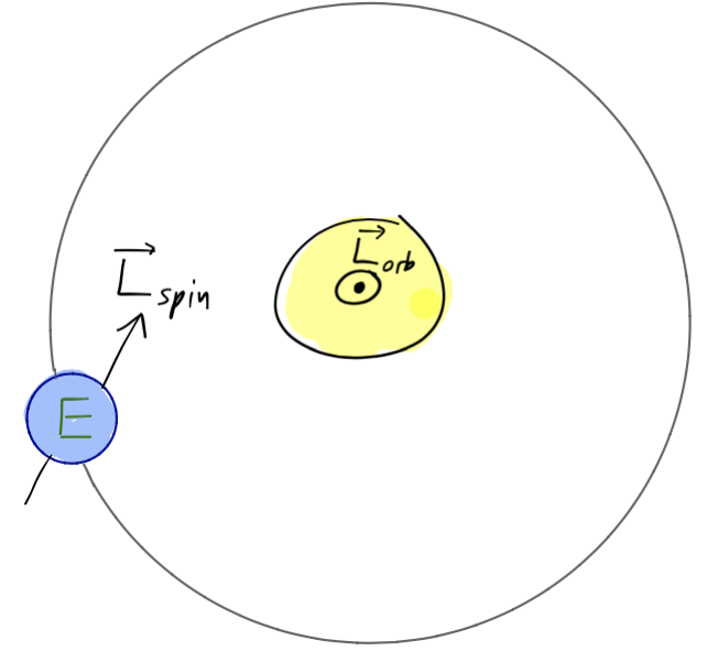
Fun fact #1: there is actually a small net torque on the Earth's spin from the Sun and Moon, mainly because the Earth isn't perfectly spherical. This causes the precession of the equinoxes, which is a small change in the Earth's orientation relative to the stars. Currently the North pole is roughly pointed towards Polaris (the "North star"), but due to the precession it will be shifted away eventually; in about a thousand years, Gamma Cephei will become the closest star to the North pole.
Fun fact #2: when you study quantum mechanics, you will see that the motion of an electron around a proton can be divided similarly into orbital and spin components which are approximately conserved (in a quantum mechanical sense) in the absence of external influence. This division turns out to be crucial for an accurate description of the observed energy levels of the hydrogen atom, for example.