Introduction

Welcome to Physics 5250!

Syllabus

We went over the syllabus at the start of class briefly. Make sure you read it yourself; you're responsible for knowing everything on there! The syllabus is subject to change if needed, but I will tell you in class, by e-mail, and on the website when anything changes.

Overview

Briefly, the list of topics we'll be covering this semester (as time allows):

1. Formalism of QM
2. The Schrodinger equation, quantum dynamics
3. Symmetries and conservation laws
4. Spin and angular momentum
5. Hydrogen atom fine and hyperfine structure
6. Perturbation theory
7. Identical particles

This material is all covered in chapters 1-4 of Sakurai, with a little bit of chapters 5 and 7 depending on how far we get.

Introduction

Since we're going to be digging into a lot of the formalism of quantum mechanics in this course, I want to start (as Sakurai's book does) with some experimental results first. What evidence is there that we live in a quantum mechanical world?

What do I mean by "a quantum mechanical world", anyway? As you know, the largest earth-shaking departures from our classical sensibilities are particle-wave duality, and the replacement of absolute determinism with probabilities. The historical development of all of these ideas is a long and complicated story, so I won't attempt to trace it; but there are some nice experiments we can look at to illustrate the concepts.

The double-slit experiment

The double-slit experiment is a classic example of particle-wave duality. The setup is simple: a barrier with two gaps in it, a source, and a detector. Famously, this experiment was carried out on light by Thomas Young in the early 1800s, an important demonstration that light propagates as a wave.

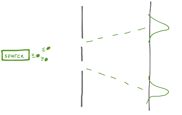
Classically, there are two versions of the experiment we can set up. If the source emits particles - macroscopic ones, like bullets for example - then after many trials, we'll find a bimodal distribution, with most of the impacts tightly distributed around the two straight-line paths from the source to the detector through the gaps.

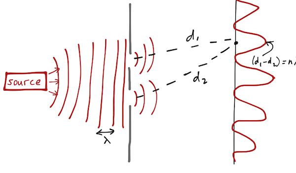
On the other hand, if our source emits a wave (using water as a medium, let's say, or light as Young showed), then the wave encounters both slits, diffracts from them, and we expect to find an interference pattern at the detector, with peaks if the difference in length traveled from the two slits is equal to \( n \lambda \), and troughs if the difference is \( (n+1/2) \lambda \).

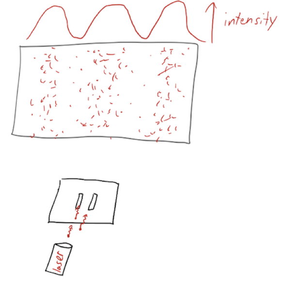
So naturally, the question arises: are fundamental particles like waves, or are they like bullets? Of course, you know that the answer is that they are both particles and waves, depending on circumstances! If we run the double-slit experiment with an extremely low source intensity, we will see individual point-like particle detections on our screen, but the intensity of the arriving particles will show the characteristic interference pattern of a wave source.

Richard Feynman, who played a large role in promoting the double-slit experiment using electrons and its variations, called it "the heart of quantum mechanics". (By the way, if you've never seen a video of this experiment, you should watch it: https://www.youtube.com/watch?v=I9Ab8BLW3kA#t=5m46s.)

So electrons are particles - we clearly see their individual impacts on the screen - and they are waves, as evidenced by the interference pattern that builds up. There are lots of interesting variants on this experiment involving measurements and quantum mechanics, but we won't go into that just yet.

Lifetime of excited atoms

One of the hardest things for a classical physicist to let go of is determinism; at the quantum level, we cannot predict the outcome of our experiment with certainty, only probabilities of outcomes!

Here's another simple experiment: start with a beam of atoms, which we've carefully prepared in the ground state. A laser is tuned to raise them to an excited state; a detector watches for the light from the reverse transition.

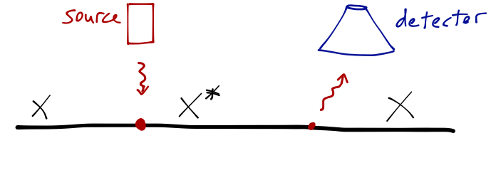
If you happen to have limitless funding and an army of graduate students, you can suppress all the sources of systematic error; you can make sure your laser energy is known precisely, that your photon detector is very efficient, that your timing measurements are accurate down to the picosecond. What will you find? Your lifetime measurements will come in one atom at a time:

• 14.243(2) ns
• 22.109(3) ns
• 8.420(2) ns

and so on. If you wait awhile to build up a distribution of results, this is what you might see:

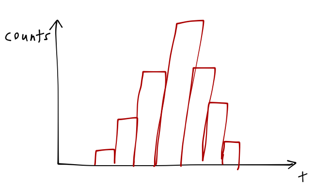
The variance of your results for the lifetime \( \tau \) is not an experimental error; you can change the properties of your source, laser, or detector, and you will find that you always measure the same distribution. The uncertainty in the decay lifetime is a fundamental property of the atomic state.

This illustrates something else important about the quantum mechanical world: it contains unavoidable randomness, but random doesn't mean we can't predict anything: properties of distributions of random events are still perfectly predictable, as here.

In fact, the energy \( E \) of our excited state isn't perfectly precise either; if we measure the frequency of the incoming photons instead of the timing, we will find a small variation \( \Delta E \) too. The energy of the excited state and its lifetime are related; if we try for several different atoms or excited states, we will always find that the variations satisfy the relation

\[ \begin{aligned} \Delta E \Delta \tau \geq \hbar / 2 \end{aligned} \]

where \( \hbar = h/2\pi \) is the usual "reduced Planck's constant". This formula is the energy-time uncertainty relation, which you have seen before and which we will return to later in the class. The main points to take away here are: first, we cannot predict the outcome of a single experiment at the quantum level; and second, we cannot know everything simultaneously about a quantum system, here the lifetime and energy of an excited atomic state.

(Side note: this explanation is a little prosaic. The energy-time uncertainty relation is not really on the same footing as the momentum-position one, since we are doing non-relativistic quantum mechanics and time doesn't behave the same way as space, as we'll see. If one studies the problem carefully including relativity, the basic point holds true: the irreducible width of the energy distribution for a particle's decay is related to its decay lifetime as \( \Delta E \sim \hbar / \tau \). This relation can be viewed as a manifestation of the uncertainty principle.)

One fun aside before we move on. The relation between energy and time uncertainty isn't all bad news; in fact, particle physicists exploit this relationship all the time. The \( Z \) boson, for example, decays so rapidly that we could never hope to perform a timing experiment like the one we set up above. But its extremely short lifetime implies a large uncertainty in its energy, and indeed if we measure the energy of the lepton pair that a \( Z \) boson decays into and plot the distribution, this is what we see:

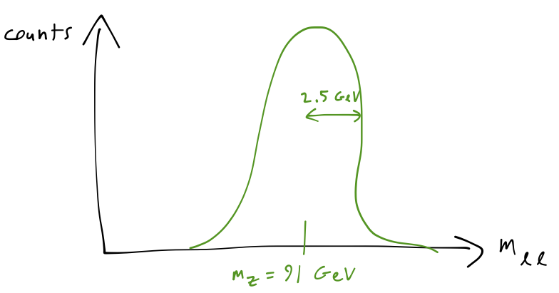
The uncertainty in the \( Z \) energy, known as its width, is measured experimentally to be about 2.5 GeV, which means that its lifetime is about 2.6 \( \times \) \( 10^{-13} \) ps - a hopeless measurement indeed!

The Stern-Gerlach apparatus

One more experiment, this time one that you're probably much less familiar with: the Stern-Gerlach experiment. We start with a beam of atoms; we'll specify silver atoms this time, since silver has a single unbound valence electron, which makes it act like a very heavy free electron. In particular, the magnetic moment \( \boldsymbol{\mu} \) of the silver atom is the same as the magnetic moment of an electron, which is proportional to the spin \( \mathbf{S} \) of the electron,

\[ \begin{aligned} \boldsymbol{\mu} \propto \mathbf{S}. \end{aligned} \]

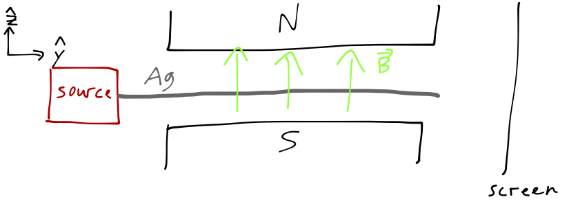
We pass our beam of silver atoms through a magnetic field, oriented in the \( \hat{z} \) direction as pictured, and then look for their locations on a distant screen in the \( \hat{y} \) direction. As you may remember, the potential energy of a magnetic moment interacting with a magnetic field \( \mathbf{B} \) is equal to \( U = -\boldsymbol{\mu} \cdot \mathbf{B} \), so that the silver atoms will feel a force in the \( \hat{z} \) direction,

\[ \begin{aligned} \mathbf{F}_z = \frac{\partial}{\partial z} (\boldsymbol{\mu} \cdot \mathbf{B}) \approx \mu_z \frac{\partial B_z}{\partial z}, \end{aligned} \]

assuming the other components of the \( \mathbf{B} \)-field are negligible. Now, if the electron behaves like a classical spinning object, then we should expect the \( z \) component of its magnetic moment to vary between \( -|\boldsymbol{\mu}| \) and \( +|\boldsymbol{\mu}| \) continuously, as the orientation of the spin axis changes. This would give us a continuous band of impacts on the screen between the two extreme values. (We're assuming (which happens to be true) that the silver atoms are heavy enough here that we can treat their motion classically.) What we actually see is two well-separated spots:

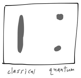
The position of the spots allows us to work backwards to determine the \( \hat{z} \)-component of the electron spin: \( S_z = \pm \hbar/2 \). So the electron's spin cannot vary continuously, it is quantized to two discrete values. It'll be awhile before we get too deep into the implications of spin quantization, but we can already see some more interesting things by chaining together Stern-Gerlach devices to make new experiments.

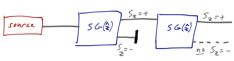
We can think of a single Stern-Gerlach apparatus as a box that splits an incoming beam into two outgoing ones which are pure spin-up (\( S_z = +\hbar/2 \)) or spin-down (\( S_z = -\hbar/2 \)) atoms. A second S-G apparatus in the \( \hat{z} \) direction is found to have no additional effect; we see only a single spot corresponding to the unblocked component.

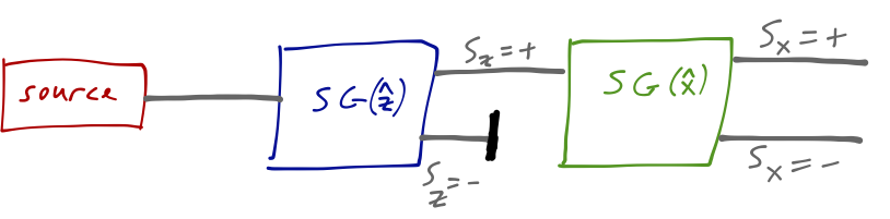
If we now rotate the second magnet so that it points in the \( \hat{x} \) direction, then we once again see two spots on the screen, corresponding to \( S_x = +\hbar/2 \) and \( S_x = -\hbar/2 \).

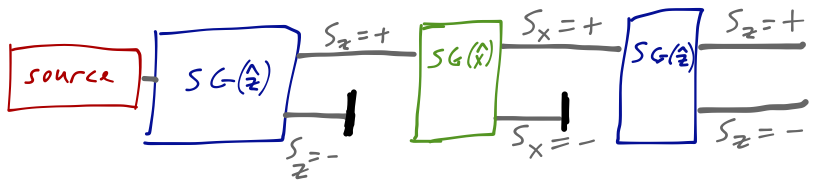
The intensity of the two spots is equal, as in the single S-G experiment. Maybe the atoms come out of the source with an initial distribution of 50% spin-up and 50% spin-down along each axis? That would explain this result, but now if we add one more magnet in the \( \hat{z} \) direction and block one of the \( \hat{x} \)-direction outputs, we find something truly surprising: two spots, corresponding to \( S_z = \pm \hbar/2 \)!

Even though we blocked the \( S_z = -\hbar/2 \) component, it has returned simply due to the presence of the \( \hat{x} \)-oriented magnet! Now, on its own this isn't ironclad proof of quantum behavior: after all, a magnetic field in the \( \hat{x} \) direction will cause the precession of a classical magnetic moment around the \( \hat{z} \) axis. For things to get weird, we have to carry out two other very similar experiments:

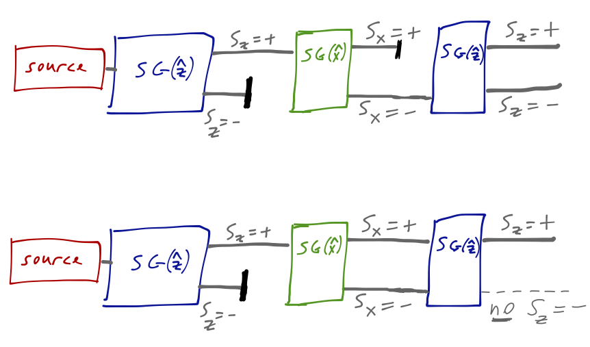
In the top configuration, we block the \( S_z = +\hbar/2 \) component; the outcome from the final \( \hat{z} \) device is the same. But if we unblock both components (this requires recombining into a single beam, which we could do with e.g. another S-G device oriented backwards), then the effect of the middle analyzer is to do nothing at all.

But now we have something really interesting! The rules of probability tell us that the outcome of the third experiment should be given by summing conditional probabilities in the following way:

\[ \begin{aligned} p(S_z = -) = p(S_z = - | S_x = +) p(S_x = +) + p(S_z = - | S_x = -) p(S_x = -) \end{aligned} \]

Every number on the right-hand side of this equation is 50%, from the other versions of the experiment above. But the left-hand side, experimentally, is zero! Aside from discarding some very fundamental axioms of probability, there is only one other way to reconcile these experiments: we must allow both intermediate states to exist at once.

(Note: there was an equation here that made use of the quantity \( p(S_x = +\ \textrm{and}\ S_x = -) \), but that was sort of wrong and misleading. The point is that the above equation doesn't work: the whole is not equal to the sum of the parts, which is characteristic of interference. See the discussion of polarized light in Sakurai or the beginning of lecture two for more discussion.)

Next time: lots of math!