Last time, we went through some motivating experimental examples, finishing with the Stern-Gerlach experiment. Aside from the quantization of spin (magnetic moments) which is immediately evident from the simplest version of the experiment, we argued that superposition effects are evident when we start chaining them together:
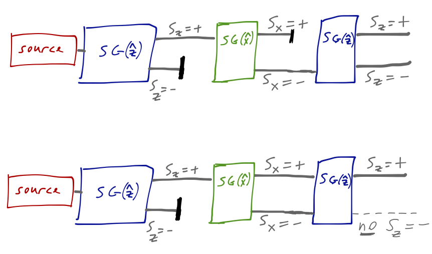
The disappearance of the \( S_z = -\hbar/2 \) component when we unblock the \( S_x = +\hbar/2 \) output of the middle Stern-Gerlach analyzer is a signature interference effect. Since all of the outputs of this experiment are probabilistic, the statement that the probability observed is different in the "combined" experiment with both outputs unblocked is best written as
\[ \begin{aligned} p(S_z = - | S_x = +\ \textrm{or}\ S_x = -) \neq p(S_z = - | S_x = +) + p(S_z = - | S_x = -). \end{aligned} \]
As I explained last time, this is suggestive of superposition, because for any two events \( A \) and \( B \) in classical probability theory, we have
\[ \begin{aligned} p(A\ \textrm{or}\ B) = p(A) + p(B) - p(A\ \textrm{and}\ B). \end{aligned} \]
so we can get destructive contributions if we allow the last term. The actual equations that I wrote out last time playing off this relation were not formulated very well, and in particular ignored the very important fact that the state was \( S_z = + \) before we went through the \( SG(\hat{x}) \) analyzer - which would lead to some very unwieldy compound conditional probabilities. Besides, we know that in quantum mechanics we work with probability amplitudes \( \psi \), which we have to square to get probabilities, schematically
\[ \begin{aligned} p(A) = |\psi(A)|^2 \end{aligned} \]
so the correct, quantum version of the superposition statement above is
\[ \begin{aligned} p_{\rm quantum}(A\ \textrm{or}\ B) = |\psi(A) + \psi(B)|^2 = p(A) + p(B) + 2\textrm{Re}(\psi^\star(A) \psi(B)), \end{aligned} \]
which is not quite the same (and good thing; you may also recall that the quantity \( p(A\ \textrm{and}\ B) \) doesn't make any sense in quantum mechanics if \( A \) and \( B \) are two possible outcomes of the same measurement!) Anyway, mea culpa if you tried to follow the math through last time, but this was only meant to motivate and we're about to get rigorous.
First, we have one more piece of motivation to squeeze out of Stern-Gerlach, from thinking about how to represent the quantum state (i.e. probability amplitude) in our experimental apparatus. Since the outcome of a Stern-Gerlach experiment is binary (spin-up or spin-down), we can use a two-dimensional vector space to represent the states. For example, we can use the \( \hat{z} \) direction experiment to establish basis vectors,
\[ \begin{aligned} S_z = +\hbar/2 \Rightarrow \left(\begin{array}{c}1\\0\end{array}\right) \\ S_z = -\hbar/2 \Rightarrow \left(\begin{array}{c}0\\1\end{array}\right). \end{aligned} \]
Given this choice, to reproduce all experimental results the \( S_x \) spin orientations should be expressed as
\[ \begin{aligned} S_x = +\hbar/2 \Rightarrow \frac{1}{\sqrt{2}} \left(\begin{array}{c}1\\1\end{array}\right) \\ S_x = -\hbar/2 \Rightarrow \frac{1}{\sqrt{2}} \left(\begin{array}{c}-1\\1\end{array}\right) \end{aligned} \]
In this abstract vector space, passing our beam through a Stern-Gerlach device and blocking one of the output components is exactly a projection along the given direction. It's easy to see in these terms that even after projecting only the \( S_z = +\hbar/2 \) component out, the subsequent projection on the \( S_x = +\hbar/2 \) direction will have both \( \hat{z} \) spin components present.
We've been forgetting about the third direction, \( S_y \). There should be nothing special about the \( \hat{x} \) direction versus \( \hat{y} \), of course - and indeed if we run the experiment above using \( \hat{y} \) instead of \( \hat{x} \), we get the same results. But it seems like we've used up our mathematical freedom in defining the \( S_x \) states! Moreover, we know that \( S_x \) and \( S_y \) have to be distinct, since obviously we expect the same results yet again if we run the sequential S-G experiment in the \( \hat{x} \) and \( \hat{y} \) directions.
The only way out is to enlarge the space by allowing the vector components to be complex; then
\[ \begin{aligned} S_y = \pm \hbar/2 \Rightarrow \frac{1}{\sqrt{2}} \left(\begin{array}{c}1\\ \pm i\end{array}\right). \end{aligned} \]
This is still sort of hand-waving, and if you're confused, I invite you to read the same description in Sakurai, which also includes a discussion of polarization of light which you may find helpful. But this is meant to be motivational, not rigorous, and the key point is that complex numbers are an essential ingredient of quantum mechanics.
Hilbert spaces
(Please note that my presentation of Hilbert spaces will be fairly practical and physics-oriented. If you have a strong math background and are interested in a more rigorous treatment, I direct you to this nice set of lecture notes from N.P. Landsman. The textbook "Analysis" by Elliott Lieb and Michael Loss was also recommended to me by a previous student.)
In your undergraduate quantum class, you may have focused on manipulation of wavefunctions, but the language of quantum mechanics is that of complex vector spaces. There are two reasons to prefer the more abstract vector-space description over wave mechanics:
- Finite-dimensional spaces - the wavefunction is a continuous distribution, but some important quantum systems only have a finite number of states, e.g. spin.
- Operators - translating classical observables into operators (in terms of \( \hat{x} \) and \( \hat{p} \)) is a mysterious procedure, and not every quantum observable has a classical starting point (once again, spin turns out to be a good example.)
Specifically, the structure we need is known as a Hilbert space. A Hilbert space is a vector space which has two additional properties:
- It has an inner product, which is a map that takes two vectors and gives us a scalar (a real or complex number.)
- All Cauchy sequences are convergent. (This isn't a math class, so we won't dwell on this property, but roughly, it guarantees that there are no "gaps" in our space.)
You're familiar with \( \mathbb{R}^n \) and \( \mathbb{C}^n \), i.e. the set of coordinate vectors in \( n \)-dimensional space; these are Hilbert spaces, with the inner product easily defined as the usual vector dot product. But remember, we need a language which is valid for both finite and infinite dimensionality; defining the inner product is a little trickier in the latter case.
Before we proceed with our study of Hilbert spaces, some notation. We will use the "bra-ket" notation introduced by Paul Dirac. Vectors in the Hilbert space \( \mathcal{H} \) will be written as "kets",
\[ \begin{aligned} \ket{\alpha} \subset \mathcal{H}. \end{aligned} \]
(I may use the words "vector" and "ket" interchangeably, but I'll try to stick to "ket".) Adding two kets gives another ket, and addition is both commutative and associative, i.e.
\[ \begin{aligned} \ket{\alpha} + \ket{\beta} = \ket{\beta} + \ket{\alpha} \\ \ket{\alpha} + (\ket{\beta} + \ket{\gamma}) = (\ket{\alpha} + \ket{\beta}) + \ket{\gamma} \end{aligned} \]
A Hilbert space, as a vector space, includes the idea of a scalar product: the product of a number \( c \) (also known as a scalar) with a ket is another ket, satisfying the following rules:
\[ \begin{aligned} (c_1 + c_2) \ket{\alpha} = c_1 \ket{\alpha} + c_2 \ket{\alpha} \\ c_1 (c_2 \ket{\alpha}) = (c_1 c_2) \ket{\alpha} \\ c (\ket{\alpha} + \ket{\beta}) = c \ket{\alpha} + c \ket{\beta} \\ 1 \ket{\alpha} = \ket{\alpha} \end{aligned} \]
Part of the definition of our vector space is what kind of number \( c \) is. For quantum mechanics, we will deal exclusively with complex Hilbert spaces, so \( c \) is complex (\( c \in \mathbb{C} \).)
We define a special ket called the null ket \( \ket{\emptyset} \), which has the properties
\[ \begin{aligned} \ket{\alpha} + \ket{\emptyset} = \ket{\alpha}\\ 0 \ket{\alpha} = \ket{\emptyset} \end{aligned} \]
Notice that thanks to the scalar multiplication rule, it's easy to see that any ket \( \ket{\alpha} \) has a corresponding inverse \( \ket{-\alpha} \), so that \( \ket{\alpha} + \ket{-\alpha} = \ket{\emptyset} \); and from our scalar product rules, \( \ket{-\alpha} = -\ket{\alpha} \).
Although we need a null ket for everything to be well-defined, since it's just equal to \( 0 \) times any ket, I'll typically just write "0" even for quantities that should be kets for simplicity. This is also to avoid confusion with kets that we want to label as \( \ket{0} \) which are just the ground state of some system and are not null.
Any set of vectors \( {\ket{\lambda_i}} \) is said to be linearly independent if the equation
\[ \begin{aligned} c_1 \ket{\lambda_1} + c_2 \ket{\lambda_2} + ... + c_n \ket{\lambda_n} = 0 \end{aligned} \]
has no solution, except the trivial \( {c_i = 0} \). I will state without proof that for an \( N \)-dimensional Hilbert space, we can find a set of \( N \) such vectors which constitute a basis, and any vector at all can be written as a sum of the basis vectors,
\[ \begin{aligned} \ket{\alpha} = \sum_{i=1}^N \alpha_i \ket{\lambda_i} \end{aligned} \]
for some set of complex coefficients \( \alpha_i \). (Note that I'm implcitly assuming finite dimension here, but in fact we can easily extend the idea of a basis to an infinite-dimensional \( \mathcal{H} \). We'll return to this point later.)
The inner product
Our defining property to have a Hilbert space was the inner product. An inner product is a map which takes two vectors (kets) and returns a scalar (complex number):
\[ \begin{aligned} (,): \mathcal{H} \times \mathcal{H} \rightarrow \mathbb{C} \end{aligned} \]
This is where we introduce the other half of our new notation: we define an object called a bra, which is written as a backwards-facing ket like so: \( \bra{\alpha} \). We need the new notation because the order of the two vectors in the product is important!
Some references (including Sakurai) will talk about the "bra space" as a "dual vector space" to our original Hilbert space, and there's nothing wrong with such a description, but don't get misled into thinking there's some big, important difference between "bra space" and "ket space". There's really just one Hilbert space \( \mathcal{H} \) that we're interested in, and bras are a notational convenience. In fact, we have a one-to-one map (the book calls this a "dual correspondence") from kets to bras and vice-versa:
\[ \begin{aligned} \ket{\alpha} \leftrightarrow \bra{\alpha} \\ c_\alpha \ket{\alpha} + c_\beta \ket{\beta} \leftrightarrow c_\alpha^\star \bra{\alpha} + c_\beta^\star \bra{\beta}. \end{aligned} \]
Notice that the duality is not quite linear; the dual to (scalar times ket) is a bra times the complex conjugate of the scalar. This is, again, a notational convenience, but one you should remember!
The upshot of all this notation is that we can rewrite the inner product of two kets as a product of a bra and a ket:
\[ \begin{aligned} (\ket{\alpha}, \ket{\beta}) \equiv \sprod{\alpha}{\beta}. \end{aligned} \]
In this notation, the inner product has the following properties:
- Linearity (in the bras):
- \( (c\bra{\alpha}) \ket{\beta} = c \sprod{\alpha}{\beta} \), and
- \( (\bra{\alpha_1} + \bra{\alpha_2}) \ket{\beta} = \sprod{\alpha_1}{\beta} + \sprod{\alpha_2}{\beta} \)
- Linearity (in the kets):
- \( \bra{\alpha} (c \ket{\beta}) = c \sprod{\alpha}{\beta} \), and
- \( \bra{\alpha} (\ket{\beta_1} + \ket{\beta_2}) = \sprod{\alpha}{\beta_1} + \sprod{\alpha}{\beta_2} \)
- Conjugate symmetry: \( \sprod{\alpha}{\beta} = \sprod{\beta}{\alpha}^\star \)
- Positive semi-definiteness: \( \sprod{\alpha}{\alpha} \geq 0 \).
Now you can see the two advantages of the bra-ket notation as we've defined it. First, because of property 3 the order of the vectors matters in the scalar product, unlike the ordinary vector dot product; dividing our vectors into bras and kets helps us to keep track of the ordering. Second, including the complex conjugate in the duality transformation means that we have both linearity properties 1 and 2 simultaneously; if we just worked with kets, the inner product would be linear in one argument and anti-linear (requiring a complex conjugation) in the other.
Hopefully you're not too confused by the notation at this point! A shorthand way to remember the difference between bras and kets is just to think of the bra as the conjugate transpose of the ket vector.
A few more things about the inner product. First, we say that two kets \( \ket{\alpha} \) and \( \ket{\beta} \) are orthogonal if their inner product is zero,
\[ \begin{aligned} \sprod{\alpha}{\beta} = \sprod{\beta}{\alpha} = 0 \Rightarrow \ket{\alpha} \perp \ket{\beta}. \end{aligned} \]
In case property 4 looks strange to you, notice that property 3 guarantees that the product of a ket with itself \( \sprod{\alpha}{\alpha} \) is always real. Since it is both real and positive, we can always take the square root of this product, which we call the norm of the ket:
\[ \begin{aligned} ||\alpha|| \equiv \sqrt{\sprod{\alpha}{\alpha}}. \end{aligned} \]
(The double straight lines is standard mathematical notation for the norm, which I'll use when it's convenient.) We can use the norm to define a normalized ket, which we'll denote with a tilde, by
\[ \begin{aligned} \ket{\tilde{\alpha}} \equiv \frac{1}{||\alpha||} \ket{\alpha}, \end{aligned} \]
so that \( \sprod{\tilde{\alpha}}{\tilde{\alpha}} = 1 \). (The only ket we can't normalize is the null ket \( \ket{\emptyset} \), which also happens to be the only ket with zero norm.) Normalized states are more than a convenience; they will, in fact, be the only allowed physical states in a quantum system. The reason is that if we work exclusively with normalized states, then the inner product becomes a map into the unit disk, and the absolute value of the inner product maps into the unit interval \( [0,1] \). This will (eventually) allow us to construct probabilities using the inner product.
Some concrete examples
Most of this discussion should have looked somewhat familiar to you, because most vector spaces you're familiar with are in fact Hilbert spaces. Ordinary coordinate space \( \mathbb{R}^3 \) is a Hilbert space; its inner product is just the dot product \( \vec{a} \cdot \vec{b} \), and the norm is just the length of the vector. (Note that because this is a real space, there's no difference between bras and kets, and the order in the inner product doesn't matter.) You can convince yourself that all of the abstract properties we've defined above hold for this space.
What about an infinite-dimensional Hilbert space, which we know we'll need to describe quantum wave mechanics? A simple example is given by the classical, vibrating string of length \( L \). Although the string has finite length, to describe its position we need an infinite set of numbers \( y(x) \) on the interval from \( x=0 \) to \( x=L \).
If we take our string and secure it between two walls with the boundary conditions \( y(0) = y(L) = 0 \), then we know that its configuration \( y(x) \) can be expanded as a Fourier series containing only sines:
\[ \begin{aligned} y(x) = \sum_{n=1}^{\infty} c_n \sin \left( \frac{n\pi x}{L} \right). \end{aligned} \]
This is nothing but a Hilbert space: the basis kets are given by the infinite set of functions \( \ket{n} = \sin (n\pi x /L) \). We can define an inner product in terms of integration:
\[ \begin{aligned} \sprod{f}{g} \equiv \frac{2}{L} \int dx\ f(x) g(x). \end{aligned} \]
With this definition, the sine functions aren't just any basis, they are an orthonormal basis: \( \sprod{m}{n} = \delta_{mn} \). (If you haven't seen it before, \( \delta_{mn} \) is the Kronecker delta, a special symbol which is equal to 1 when \( m=n \) and 0 otherwise.)
The Cauchy-Schwarz inequality
Stepping back to the more abstract level, there are some useful identities that we can prove using only the general properties of Hilbert space we've defined above. One which we will find particularly useful is the Cauchy-Schwarz inequality,
\[ \begin{aligned} \sprod{\alpha}{\alpha} \sprod{\beta}{\beta} \geq |\sprod{\alpha}{\beta}|^2. \end{aligned} \]
I'll go through the proof now, just to show you a little practice in manipulating vectors. Obviously if either ket is the null ket, we just have \( 0=0 \), so we can assume everything is non-zero.
Where do we go next? Once again, if we think of coordinate space \( \mathbb{R}^n \), the Cauchy-Schwarz inequality states that \( (\vec{a} \cdot \vec{b})^2 \leq |a|^2 |b|^2 \). In this case, we can rewrite the inner product in terms of the angle between the vectors,
\[ \begin{aligned} \vec{a} \cdot \vec{b} = |a| |b| \cos \theta. \end{aligned} \]
This makes the proof trivial, but it also tells us that the inequality is saturated (becomes an equality) only if the two vectors point in the same direction. This suggests that we should start by isolating the part of \( \ket{\alpha} \) which is orthogonal to \( \ket{\beta} \).
I left completing the proof for arbitrary Hilbert space to you at this point, as an exercise; I'll give the answer next time.