Last time, we started talking about the possibility of continuous operators, which have an infinite number of outcomes - e.g. observables like position \( \hat{x} \). Based on the postulates of QM, we need a correspondingly infinite Hilbert space to describe such operators. Fortunately, almost all of the formalism we have developed so far for Hilbert spaces is unaffected by this distinction! There are two general replacements we will have to make:
- Sums should be replaced with integrals, e.g. in the completeness relation
\[ \begin{aligned} \hat{1} = \int d\xi\ \ket{\xi}\bra{\xi} \end{aligned} \]
- Kronecker delta functions should be replaced with Dirac delta functions, e.g. in the orthogonality relation
\[ \begin{aligned} \sprod{\xi}{\xi'} = \delta(\xi - \xi') \end{aligned} \]
We'll be using the delta function a lot and it is a somewhat mysterious object (it's technically a distribution, not a function!), so let's study some of its properties.
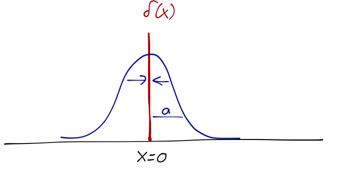
The Dirac delta function is defined to be zero at every point, except where its argument is zero. Although it is only non-zero for an infinitesmal span, the area under the delta function is constant:
\[ \begin{aligned} \int dx\ \delta(x) = 1. \end{aligned} \]
If we integrate another function times the delta function, we "pick out" the one point where the argument of \( \delta(x) \) is zero:
\[ \begin{aligned} \int dx\ \delta(x-a) f(x) = f(a). \end{aligned} \]
The delta function "collapses" the integral, selecting out a single value of the function; this is similar to what the Kronecker delta does to sums. Note that I haven't included limits of integration; these identities are true when we integrate over any integral that contains the non-zero part of \( \delta(x) \).
As I mentioned, strictly speaking \( \delta(x) \) is not a function; you should be very careful with its interpretation when it's not safely under an integral! When in doubt, you can fall back on a more rigorous definition in terms of a limit of a set of functions; there's more than one definition, but one useful construction is a Gaussian distribution with vanishing width:
\[ \begin{aligned} \delta(x) = \lim_{a \to 0} \frac{1}{\sqrt{\pi} a} \exp \left( - \frac{x^2}{a^2} \right). \end{aligned} \]
You can verify that this definition recovers the integral properties we found above. We can also use it to derive some more useful properties:
\[ \begin{aligned} \delta(-x) = \delta(x) \\ \delta'(-x) = -\delta'(x) \\ x \delta'(x) = -\delta(x) \\ \delta (ax) = \frac{1}{|a|} \delta(x) \\ \delta(x^2 - a^2) = \frac{1}{2|a|} [ \delta(x+a) + \delta(x-a) ] \end{aligned} \]
More generally, for any function inside the \( \delta \) we have
\[ \begin{aligned} \delta(f(x)) = \sum_i \frac{\delta(x-x_i)}{|f'(x_i)|} \end{aligned} \]
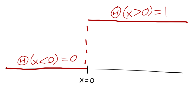
where \( x_i \) are the roots of \( f(x) \), i.e. \( f(x_i) = 0 \). (If you want to see why this last property is true, use the limit representation and Taylor expand about the roots.) One more special function: if we integrate the Dirac delta from \( -\infty \) to \( x \), we get either 0 or 1, depending on whether our integration includes \( x=0 \). This defines the Heaviside step function \( \Theta(x) \),
\[ \begin{aligned} \Theta(x) \equiv \int_{-\infty}^x dx'\ \delta(x') = \begin{cases} 0, & x<0; \\ 1, & x\geq 0 \end{cases}. \end{aligned} \]
The other distinction between discrete and continuous operators is that we can no longer use finite matrices and vectors to represent operators and states. We can still expand an arbitrary state vector in a continuous basis,
\[ \begin{aligned} \ket{\psi} = \int d\xi\ \ket{\xi} \sprod{\xi}{\psi}. \end{aligned} \]
We simply write the infinite set of coefficients \( \sprod{\xi}{\psi} \) as a single continuous function,
\[ \begin{aligned} \sprod{\xi}{\psi} \rightarrow \psi(\xi). \end{aligned} \]
You can see that we're getting close to recovering the wavefunction of wave mechanics! Let's add the last missing piece by considering our first concrete example of a continuous operator: the position operator.
The position operator
We'll start by working in one dimension; it will be easy to generalize to three. In one dimension, we define the position operator \( \hat{x} \), an observable corresponding to the position of a particle. Position is continuous, so we have an infinite basis given by
\[ \begin{aligned} \hat{x} \ket{x} = x \ket{x} \end{aligned} \]
leading to the matrix elements
\[ \begin{aligned} \bra{x'} \hat{x} \ket{x} = x \delta(x'-x) \end{aligned} \]
and an arbitrary state can be written as
\[ \begin{aligned} \ket{\psi} = \int_{-\infty}^\infty dx\ \ket{x}\sprod{x}{\psi} = \int_{-\infty}^\infty dx\ \psi(x) \ket{x}. \end{aligned} \]
Just like any other observable, position satisfies the "collapse" postulate; if we measure the position of a particle and find it to be \( x \), then the state vector collapses from \( \ket{\psi} \rightarrow \ket{x} \). Of course, in reality even the best position measurements have some uncertainty; the best we can do in practice is pinpoint the position to be within the interval \( [x-\Delta, x+\Delta] \) for some measurement error \( \Delta \).
We can imagine the state collapse after this measurement to be represented by projection onto the set of \( \hat{x} \) eigenstates within this small space interval. We can go on to construct an operator associated with this projection as an outer product:
\[ \begin{aligned} \hat{M}(x, \Delta) = \int_{x-\Delta}^{x+\Delta} dx'\ \ket{x'} \bra{x'} = \int_{-\infty}^\infty dx'\ \ket{x'} \bra{x'} (\Theta(x'-x+\Delta) - \Theta(x'-x-\Delta)) \end{aligned} \]
where I've used the difference of step functions to construct a "boxcar function" that selects the chosen interval. Its matrix element between two position eigenstates is
\[ \begin{aligned} \bra{x'} \hat{M}(x, \Delta) \ket{x''} = \int_{-\infty}^\infty dx'''\ \sprod{x'}{x'''} \sprod{x'''}{x''} \left( \Theta(x'''-x+\Delta) - \Theta(x'''-x-\Delta) \right) \\ = \delta(x'-x'') \left( \Theta(x'-x+\Delta) - \Theta(x'-x-\Delta) \right). \end{aligned} \]
This means that for an arbitrary physical state,
\[ \begin{aligned} \bra{\psi} \hat{M}(x, \Delta) \ket{\psi} = \int dx' \int dx''\ \sprod{\psi}{x'} \bra{x'} \hat{M} \ket{x''} \sprod{x''}{\psi} \\ = \int dx' \int dx''\ \sprod{\psi}{x'} \delta(x'-x'') \left( \Theta(x'-x+\Delta) - \Theta(x'-x-\Delta) \right) \sprod{x''}{\psi} \\ = \int_{x-\Delta}^{x+\Delta} dx'\ |\sprod{\psi}{x'}|^2 = \int_{x-\Delta}^{x+\Delta} dx' |\psi(x')|^2. \end{aligned} \]
So the probability to find our particle in the interval \( [x-\Delta, x+\Delta] \) is given by integrating the function \( \psi(x) \), which you should now recognize as the usual wavefunction, over that interval. This shows that we can interpret \( |\psi(x)|^2 \) as a probability density function for the \( x \) position of our particle. For example, the expectation value of an arbitrary observable which is a function only of position \( \hat{A}(\hat{x}) \) becomes
\[ \begin{aligned} \ev{\hat{A}(\hat{x})} = \int_{-\infty}^\infty dx\ A(x) |\psi(x)|^2 \end{aligned} \]
which you'll recognize as the usual definition of the expectation value over a probability distribution.
(Note: this construction is meant to emphasize the correspondence between wavefunction and probability density, not as a realistic model for experimental measurements with error! In particular \( \hat{M} \) is a projection operator, not a measurement - we'd have to be more careful to construct a measurement operator that modifies \( \hat{x} \) to only give results in a finite region. The simple-minded way to do so is just to restrict our space to \( \) instead of \( \), and then use \( \hat{x} \) as normal.)
As a pdf, \( p(x) \) should be normalized so that its integral over all \( x \) values is 1 (the probability of finding our particle anywhere at all should be 1):
\[ \begin{aligned} \sprod{\psi}{\psi} = \int_{-\infty}^\infty dx\ |\psi(x)|^2 = 1. \end{aligned} \]
This is equivalent to the statement that the norm of the state \( \sprod{\psi}{\psi} = 1 \). More generally, the inner product of two states is now also given by an integral,
\[ \begin{aligned} \sprod{\phi}{\psi} = \int_{-\infty}^\infty dx\ \sprod{\phi}{x} \sprod{x}{\psi} = \int_{-\infty}^\infty dx\ \phi^\star(x) \psi(x). \end{aligned} \]
and matrix elements between arbitrary states by a double integral:
\[ \begin{aligned} \bra{\phi} \hat{A} \ket{\psi} = \int dx \int dx'\ \sprod{\phi}{x} \bra{x} \hat{A} \ket{x'} \sprod{x'}{\psi} \\ = \int dx \int dx'\ \phi^\star(x) \bra{x} \hat{A} \ket{x'} \psi(x). \end{aligned} \]
If \( \hat{A} = \hat{A}(\hat{x}) \) is purely a function of the position operator \( \hat{x} \), then its matrix elements are \( A(x) \delta(x-x') \), and the integral collapses, giving us
\[ \begin{aligned} \ev{\hat{A}(\hat{x})} = \int_{-\infty}^\infty dx\ A(x) |\psi(x)|^2. \end{aligned} \]
This once again reinforces the notion of \( |\psi(x)|^2 \) as a probability density. But keep in mind that the fundamental quantity here is \( \psi \), not its square. The fact that quantum mechanical states are described by probability amplitudes (which square to give probabilities) is a source of much of the interesting quantum behavior we will see. In classical probability theory, if we have two events \( A \) and \( B \) which are independent (e.g. rolling 1 and 5 on two different dice at once), then the probability of joint event \( A \cap B \) is given by the product
\[ \begin{aligned} p(A \cap B) = p(A) p(B). \end{aligned} \]
On the other hand, if \( A \) and \( B \) are mutually exclusive (rolling 1 or 5 on the same die at once), then the probability of measuring either event \( A \) or event \( B \) is given by the sum,
\[ \begin{aligned} p(A \cup B) = p(A) + p(B). \end{aligned} \]
In quantum mechanics, the first rule still holds; I invoked this a couple lectures ago when we were looking at sequential projection measurements and how they affected outcomes. However, the big difference in a quantum world is that for exclusive outcomes (like, say, an electron passing through one of two openings in a screen), it's not the probabilities but the amplitudes which add:
\[ \begin{aligned} \psi(A \cup B) = \psi(A) + \psi(B), \end{aligned} \]
so that
\[ \begin{aligned} p_{\textrm{quantum}}(A \cup B) = |\psi(A) + \psi(B)|^2 = p(A) + p(B) + 2 \textrm{Re}(\psi^\star(A) \psi(B)). \end{aligned} \]
This extra interference term between exclusive events is at the core of quantum behavior, as we've seen in our specific example involving Stern-Gerlach like experiment before; but it's worth repeating in this more general and simplified way.
The momentum operator
Now, if \( \hat{A} \) is just some function of position, then the matrix elements with the position eigenkets are simple:
\[ \begin{aligned} \bra{x} \hat{A} \ket{x'} = A(x') \delta(x-x') \end{aligned} \]
and the general matrix element above collapses to a single integral. But not every operator is just a function of position! For example, we can introduce a momentum operator \( \hat{p} \), which measures the momentum of our particle (still in one dimension.)
How do we calculate \( \bra{x} \hat{p} \ket{x'} \)? It should be obvious that momentum eigenstates cannot also be position eigenstates; momentum implies movement, which is a change of position. Sakurai gives a long discussion of the relation between momentum and change in position (aka translation) in section 1.6; I want to defer that study until we get to a more detailed treatment of symmetries in quantum mechanics, so don't worry if you didn't follow that section right now. Instead I am going to start with the canonical commutation relation,
\[ \begin{aligned} [\hat{x}, \hat{p}] = i\hbar. \end{aligned} \]
Some books treat this as another postulate; you can also think of it as a definition of momentum and/or of Planck's constant,
\[ \begin{aligned} \hbar = \frac{h}{2\pi} = 1.055 \times 10^{-34}\ \mbox{J s} \end{aligned} \]
This commutator is all we need to determine what \( \hat{p} \) must look like in coordinate space. If we sandwich the commutator between an arbitrary pair of states, we have
\[ \begin{aligned} \bra{\phi} [\hat{x}, \hat{p}] \ket{\psi} = \int dx \int dx'\ \sprod{\phi}{x} \bra{x} \hat{x} \hat{p} - \hat{p} \hat{x} \ket{x'} \sprod{x'}{\psi} \\ = \int dx \int dx'\ \phi^\star(x) (x \bra{x}\hat{p}\ket{x'} - \bra{x}\hat{p}\ket{x'} x') \psi(x') \end{aligned} \]
where we can act either to the left or to the right with \( \hat{x} \), since it's an observable and therefore Hermitian. By the canonical commutation relation, this must be equal to
\[ \begin{aligned} \bra{\phi} [\hat{x}, \hat{p}] \ket{\psi} = i \hbar \sprod{\phi}{\psi} = i\hbar \int dx\ \phi^\star(x) \psi(x). \end{aligned} \]
No function of \( \hat{x} \) can satisfy this relation; basically, the matrix element we want should contain something like a Dirac delta \( \delta(x-x') \) to collapse two integrals down to one - but then the two terms in the first expression above will immediately give zero when \( x = x' \)! If you stare at the expressions long enough, you can verify that the solution to this equation must involve a derivative as the matrix element:
\[ \begin{aligned} \bra{x} \hat{p} \ket{x'} = \delta(x-x') \frac{\hbar}{i} \frac{\partial}{\partial x} \end{aligned} \]
In other words, we can write the wavefunction corresponding to \( \hat{p} \) acting on an arbitrary state as
\[ \begin{aligned} \bra{x} \hat{p} \ket{\psi} = \int dx'\ \bra{x} \hat{p} \ket{x'} \sprod{x'}{\psi} \\ = \int dx' \delta(x-x') \frac{\hbar}{i} \frac{\partial}{\partial x} \sprod{x'}{\psi} \\ = \frac{\hbar}{i} \frac{\partial \psi(x)}{\partial x}. \end{aligned} \]
Clearly, acting with momentum repeatedly just gives more derivatives, so matrix elements for powers of \( \hat{p} \) can be written as:
\[ \begin{aligned} \bra{\phi} \hat{p}{}^n \ket{\psi} = \int dx\ \phi^\star(x) \left( \frac{\hbar}{i} \frac{\partial}{\partial x} \right)^n \psi(x). \end{aligned} \]
The canonical commutation relation tells us, unsurprisngly, that \( \hat{x} \) and \( \hat{p} \) are incompatible observables; they have no simultaneous eigenstates. Applying the uncertainty relation gives us the familiar Heisenberg uncertainty principle for position and momentum,
\[ \begin{aligned} \Delta x \Delta p \geq \hbar/2. \end{aligned} \]
Of course, the momentum operator has its own orthonormal basis of state with definite momentum,
\[ \begin{aligned} \hat{p} \ket{p} = p \ket{p}. \end{aligned} \]
Given a particular physical state, we can expand it instead in momentum eigenstates:
\[ \begin{aligned} \ket{\psi} = \int dp\ \ket{p} \sprod{p}{\psi} = \int dp\ \ket{p} \tilde{\psi}(p) \end{aligned} \]
where now \( \tilde{\psi}(p) \) is the momentum-space wavefunction, denoted in my notation with a tilde. (Sometimes you'll see people use \( \phi \) for a generic momentum-space wavefunction complementary to \( \psi \); I prefer the tilde since it's more general.)
Relation between the bases
Just as in the finite-dimensional case, we can compute a change of basis from position to momentum space, or vice-versa:
\[ \begin{aligned} \sprod{x}{\psi} = \int dp\ \sprod{x}{p} \sprod{p}{\psi} \end{aligned} \]
The overlap between the two basis states isn't immediately obvious, but we can figure it out. Since we're integrating over \( p \) we want to find the function \( \sprod{x}{p} \) in momentum space. Notice that
\[ \begin{aligned} \bra{x} \hat{p} \ket{p} = p \sprod{x}{p} = \frac{\hbar}{i} \frac{\partial}{\partial x} \sprod{x}{p}. \end{aligned} \]
This is just a differential equation, which you should recognize the solution to right away:
\[ \begin{aligned} \sprod{x}{p} = \frac{1}{\sqrt{2\pi \hbar}} \exp \left( \frac{ipx}{\hbar} \right) \end{aligned} \]
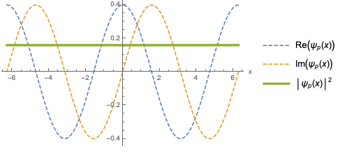
(where the normalization ensures that \( \sprod{x}{x'} = \delta(x-x') \) when we insert a complete set of \( \ket{p} \) states.) Although we're about to use this to change bases, I'll stop and point out that this also tells us what a momentum eigenstate looks like in position space: an oscillating, complex exponential which is periodic under
\[ \begin{aligned} x \rightarrow x + 2\pi \hbar / p \equiv x + 2\pi/k. \end{aligned} \]
This is called a plane wave, and the quantity \( k \) with units of inverse length is the wave number. As we would expect, the plane wave is a state which is absolutely localized in momentum space at \( p \), and is therefore completely delocalized in position space: if we calculate the mean and variance, we will find that \( \ev{\hat{x}} = 0 \) but \( \Delta x = \infty \).
Note that this is one of the examples I mentioned where you need to be cautious with delta functions and infinities! If you try to make sure the plane wave solution is normalized, you will find that
\[ \begin{aligned} \int_{-\infty}^\infty dx\ |\sprod{x}{p}|^2 = \int_{-\infty}^\infty dx\ \frac{1}{2\pi \hbar} \exp \left(\frac{ipx}{\hbar} - \frac{ipx}{\hbar} \right) = \infty \end{aligned} \]
which looks like a disaster! In fact, we can write this a bit more generally noticing that if we tried to integrate over two different momentum eigenstates, then the result is zero. (You can do this by rewriting the integral as a contour integral in the complex plane, noticing that there are no poles inside the residue, and that as long as \( p \neq p' \) the integral off the real line will be exponentially damped.) In fact, we know from our definitions in Hilbert space that we must have
\[ \begin{aligned} \sprod{p}{p'} = \delta(p-p'). \end{aligned} \]
We accept such improperly normalized states into our Hilbert space, because they are useful to think about in certain situations. In practice, any physical system will be localized to some finite region of space and we won't have to worry about this subtle divergence.
We can carry through a similar argument to go in the opposite direction, i.e. to find the position eigenstates in momentum space. It won't surprise you that the operator \( \hat{x} \) acts as a derivative in momentum space, except with the \( i \) upstairs:
\[ \begin{aligned} \bra{p} \hat{x} \ket{p'} = \delta(p-p') i\hbar \frac{\partial}{\partial p}. \end{aligned} \]
In fact, in momentum space we find exactly the same function for the product \( \sprod{x}{p} \). What we've proved is that the functions representing a particular state in position and momentum space are nothing but Fourier transforms of one another:
\[ \begin{aligned} \psi(x) = \frac{1}{\sqrt{2\pi \hbar}} \int dp\ \exp \left(\frac{ipx}{\hbar} \right) \tilde{\psi}(p) \\ \tilde{\psi}(p) = \frac{1}{\sqrt{2\pi \hbar}} \int dx\ \exp \left(\frac{-ipx}{\hbar} \right) \psi(x). \end{aligned} \]
More than one spatial dimension
Although we'll be working in one dimension for a while, there is no complication to passing to three dimensions. You'll generally see \( \vec{r} = (x,y,z) \) as the three-dimensional position vector; I'll follow Sakurai and use \( \vec{x} \). The canonical commutation relation only holds for position and momentum in the same direction; positions and/or momenta pointing in different Cartesian directions always commute. We can expand the set of commutation relations to read
\[ \begin{aligned} [x_i, x_j] = 0 \\ [p_i, p_j] = 0 \\ [x_i, p_j] = i \hbar \delta_{ij}. \end{aligned} \]
Most of our notation and work above passes through unchanged. Position eigenstates are labelled with \( \ket{\vec{x}} = \ket{x,y,z} \), and similarly for momentum. They are normalized accounting properly for all thre dimensions, i.e.
\[ \begin{aligned} \sprod{\vec{x}}{\vec{x}'} = \delta^3(\vec{x} - \vec{x}') = \delta(x-x') \delta(y-y') \delta(z-z') \end{aligned} \]
and again, similarly for momentum. Integrals for inner products etc. are now over all three dimensions. The representation of the momentum operator in position space becomes the gradient,
\[ \begin{aligned} \hat{\vec{p}} = \frac{\hbar}{i} \frac{\partial}{\partial \vec{x}} = \frac{\hbar}{i} \vec{\nabla}_x \end{aligned} \]
and the converse
\[ \begin{aligned} \hat{\vec{x}} = i\hbar \frac{\partial}{\partial \vec{p}} = i\hbar {\vec{\nabla}}_p. \end{aligned} \]
Finally, the Fourier transform relation between momentum and position space looks almost the same, but with a different normalization:
\[ \begin{aligned} \psi(\vec{x}) = \frac{1}{(2\pi \hbar)^{3/2}} \int d^3p\ \exp \left(\frac{i\vec{p} \cdot \vec{x}}{\hbar} \right) \tilde{\psi}(\vec{p}) \\ \psi(\vec{p}) = \frac{1}{(2\pi \hbar)^{3/2}} \int d^3x\ \exp \left(\frac{-i\vec{p} \cdot \vec{x}}{\hbar} \right) {\psi}(\vec{x}) \end{aligned} \]