Wave packets
As was pointed out in class, the step-function example of a localized position state that we constructed before wasn't very realistic. A more practical construction is an object known as the Gaussian wave packet. We define such a state through its position space wave function,
\[ \begin{aligned} \sprod{x}{\psi} = \psi(x) = \frac{1}{\pi^{1/4} \sqrt{d}} \exp \left( ikx - \frac{x^2}{2d^2} \right). \end{aligned} \]
To construct this state we've started with a plane wave of wave number \( k \), and then modulated it with (multiplied by) a Gaussian distribution centered at \( x=0 \) with width \( d \). The Gaussian envelope localizes our state near \( x=0 \); the real and imaginary parts of the ampltiude in \( x \) (arbitrarily taking \( d=1 \)) now look like this:
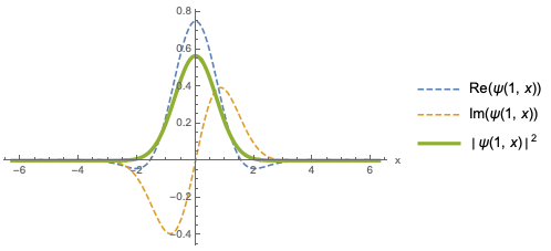
where I've overlaid the probability density \( |\psi(x)|^2 \), which is Gaussian. Clearly this looks localized, but let's actually go through the exercise of calculating the expectation values for position. The mean is given by
\[ \begin{aligned} \ev{\hat{x}} = \int_{-\infty}^\infty dx \sprod{\psi}{x} x \sprod{x}{\psi} = \int_{-\infty}^\infty dx\ |\psi(x)|^2 \\ = \frac{1}{\sqrt{\pi} d} \int_{-\infty}^\infty dx\ x \exp(-x^2/d^2) = 0 \end{aligned} \]
since the integral is odd. For \( \hat{x}^2 \), things are a little tougher:
\[ \begin{aligned} \ev{\hat{x}{}^2} = \frac{1}{\sqrt{\pi}d} \int_{-\infty}^\infty dx\ x^2 \exp(-x^2/d^2) \end{aligned} \]
Gaussian integrals such as this one crop up everywhere in physics, so let's take a slight detour to study them. We start with the most basic Gaussian integral,
\[ \begin{aligned} I(\alpha) \equiv \frac{1}{\sqrt{\pi} d} \int_{-\infty}^\infty dx\ \exp(-\alpha x^2) = \sqrt{\frac{\pi}{\alpha}}. \end{aligned} \]
The result for \( \alpha = 1 \) was originally found by Laplace, and can be elegantly derived by squaring the integral and changing to polar coordinates. This is all we need to derive the result we need above: if we take the derivative of the integral with respect to \( \alpha \), we find
\[ \begin{aligned} \frac{\partial}{\partial \alpha} \int_{-\infty}^\infty dx\ e^{-\alpha x^2} = -\int_{-\infty}^\infty dx\ x^2 e^{-\alpha x^2}. \end{aligned} \]
So
\[ \begin{aligned} \int_{-\infty}^\infty dx\ x^2 e^{-\alpha x^2} = -\frac{\partial I}{\partial \alpha} = \frac{\sqrt{\pi}}{2\alpha^{3/2}}. \end{aligned} \]
For higher even powers of \( x \), we just take more derivatives with respect to \( \alpha \); all the odd powers vanish. The general result for \( n \) even can be shown to be
\[ \begin{aligned} \int_{-\infty}^\infty dx\ x^n e^{-\alpha x^2} = \frac{(n+1)!! \sqrt{\pi}}{2^{n/2} \alpha^{(n+1)/2}}. \end{aligned} \]
where \( !! \) is the double factorial symbol, \( (n+1)!! = (n+1)(n-1)...(5)(3)(1) \).
I'll finish this example in one dimension, but as long as we're doing math, I'll remark on the generalization to multi-dimensional Gaussian integrals. With \( n \) coordinates, the most general pure Gaussian integral we can write is
\[ \begin{aligned} \int d^n x \exp \left( -\frac{1}{2} \sum_{i,j} A_{ij} x_i x_j \right) = \int d^n x \exp \left( -\frac{1}{2} \vec{x}^T \mathbf{A} \vec{x} \right) = \sqrt{\frac{(2\pi)^n}{\det \mathbf{A}}}, \end{aligned} \]
where the \( 1/2 \) is conventional, and the result is most nicely expressed by thinking of the various numbers \( A_{ij} \) as forming a matrix \( \mathbf{A} \). Using derivatives with respect to \( A_{ij} \) on this expression can similarly give us more complicated functions to integrate against, just with more algebra than the 1-d case.
Back to our wave packet: the dispersion in \( \hat{x} \) is now seen to be
\[ \begin{aligned} \ev{\hat{x}{}^2} = \frac{1}{\sqrt{\pi} d} \frac{\sqrt{\pi}d^3}{2} = \frac{d^2}{2}. \end{aligned} \]
so \( \Delta x = \sqrt{\ev{\hat{x}^2} - \ev{\hat{x}}^2} = d/\sqrt{2} \).
What about the momentum? We started with a plane wave of definite momentum \( \hbar k \), but the convolution with the Gaussian will have changed that. Being careful about the order now, we can see that the expectation value of \( \hat{p} \) is
\[ \begin{aligned} \ev{\hat{p}} = \int_{-\infty}^\infty dx\ \int_{-\infty}^\infty dx'\ \sprod{\psi}{x} \bra{x} \hat{p} \ket{x'} \sprod{x'}{\psi}\\ = \int_{-\infty}^\infty dx\ \int_{-\infty}^\infty dx'\ \psi^\star(x) \left( -i\hbar \delta(x-x') \frac{\partial}{\partial x} \right) \psi(x') \\ = \frac{-i\hbar}{\sqrt{\pi} d} \int_{-\infty}^\infty dx\ e^{-ikx - x^2/(2d^2)} \left(ik - \frac{x}{d^2} \right) e^{ikx-x^2/(2d^2)} \\ = \frac{\hbar k}{\sqrt{\pi d}} (\sqrt{\pi} d) = \hbar k \end{aligned} \]
where the second term proportional to \( x/d^2 \) is odd in \( x \) and vanishes identically. So the Gaussian convolution didn't change the mean value of the momentum from the plane wave we started with. However, there is now some dispersion in the momentum; you can verify that
\[ \begin{aligned} \ev{\hat{p}{}^2} = \frac{\hbar^2}{2d^2} + \hbar^2 k^2, \end{aligned} \]
which gives
\[ \begin{aligned} \Delta p = \frac{\hbar}{\sqrt{2} d}. \end{aligned} \]
Notice that if we try to explicitly check the uncertainty relation, we find that
\[ \begin{aligned} \Delta x \Delta p \geq \frac{1}{2} \left|\ev{[\hat{x}, \hat{p}]}\right| \\ \Rightarrow \hbar/2 \geq \hbar/2. \end{aligned} \]
Not only does our wave packet satisfy the uncertainty relation, it saturates it; we have an equality. The Gaussian wave packet is known as the minimum uncertainty wave packet because it gives the smallest product of uncertainties \( \Delta x \Delta p \).
What does the wave packet look like in terms of momentum? We can easily carry out the Fourier transform:
\[ \begin{aligned} \tilde{\psi}(p) = \int dx \sprod{p}{x} \sprod{x}{\psi} \\ = \frac{1}{\sqrt{2\pi \hbar}} \int dx\ \exp\left(\frac{-ipx}{\hbar}\right) \frac{1}{\pi^{1/4} \sqrt{d}} \exp \left(ikx - \frac{x^2}{2d^2} \right) \\ = \frac{1}{\sqrt{2\hbar d} \pi^{3/4}} \int dx\ \exp \left[ -\left(\frac{x}{\sqrt{2}d} -\frac{id(k-p/\hbar)}{\sqrt{2}}\right)^2 - \frac{d^2 (p-\hbar k)^2}{2\hbar^2}\right] \end{aligned} \]
completing the square. But this is an integral from \( -\infty \) to \( \infty \), so we can just shift the integration to the squared quantity, and we have an ordinary Gaussian integral with \( dx' = dx/(\sqrt{2}d) \). Thus:
\[ \begin{aligned} \tilde{\psi}(p) = \frac{1}{\sqrt{2\hbar d} \pi^{3/4}} \exp \left(\frac{-d^2(p-\hbar k)^2}{2\hbar^2}\right) \sqrt{2}d \int_{-\infty}^\infty dx'\ e^{-x'{}^2} \\ = \frac{1}{\pi^{1/4} \sqrt{\hbar/d}} \exp \left( \frac{-(p-\hbar k)^2}{2(\hbar/d)^2} \right). \end{aligned} \]
This is, once again, a Gaussian distribution, this time with mean value \( \hbar k \) and variance \( \hbar2/2d2 \), exactly as we found from the \( x \) wavefunction directly. You can evaluate these expectation values directly, or you can just read them off of the distribution; we know that \( |\tilde{\psi}(p)|^2 \) is a Gaussian probability density, which takes the generic form we saw previously
\[ \begin{aligned} p(\mu, \sigma) = \frac{1}{\sqrt{2\pi} \sigma} e^{-(x-\mu)^2/(2\sigma^2)} \end{aligned} \]
for mean \( \mu \) and variance \( \sigma^2 \). Notice that, unsurprisingly, the width of the momentum Gaussian packet is proportional to \( 1/d \), whereas in position space it goes as \( d \). The more we squeeze the spread of momentum states, the wider the distribution in position becomes, and vice-versa; this behavior is a consequence of the uncertainty relation. In the limit \( d \rightarrow \infty \) we recover the plane wave; a delta-function in \( p \)-space and an infinite wave in \( x \)-space.
The Hamiltonian operator
Now that we have a handle on the position and momentum operators, we can construct a number of other interesting observables from them. The most important is the Hamiltonian, \( \hat{H} \). You'll recall from classical mechanics that usually, the Hamiltonian is equal to the total energy \( T+U \), and indeed the eigenvalues of the quantum Hamiltonian operator are the energy of the system \( E \). A generic Hamiltonian for a single particle of mass \( m \) moving in some potential \( V(x) \) is
\[ \begin{aligned} \hat{H} = \frac{\hat{p}{}^2}{2m} + V(\hat{x}). \end{aligned} \]
For an eigenstate of energy, by definition the Hamiltonian satisfies the equation
\[ \begin{aligned} \hat{H} \ket{E} = E \ket{E}. \end{aligned} \]
What are the matrix elements of an arbitrary state? Well, in position space:
\[ \begin{aligned} \bra{x} \hat{H} \ket{\psi} = \int dx'\ \bra{x} \hat{H} \ket{x'} \sprod{x'}{\psi} \\ = \int dx'\ \left[ \bra{x} \frac{\hat{p}{}^2}{2m} \ket{x'} + \delta(x-x') V(x') \right] \psi(x') \\ = \int dx'\ \delta(x-x') \left[ \frac{1}{2m} \left( \frac{\hbar}{i} \frac{\partial}{\partial x}\right)^2 + V(x') \right] \psi(x') \\ = \left[ -\frac{\hbar^2}{2m} \frac{\partial^2}{\partial x^2} + V(x) \right] \psi(x). \end{aligned} \]
If the state \( \ket{\psi} \) is an energy eigenstate, then we also have \( \bra{x} \hat{H} \ket{\psi, E} = E \sprod{x}{\psi_E} \), or
\[ \begin{aligned} -\frac{\hbar^2}{2m} \frac{\partial^2 \psi_E}{\partial x^2} + V(x) \psi_E(x) = E \psi_E(x), \end{aligned} \]
which you'll recognize as the (time-independent) Schrödinger equation.
If we have a free particle, i.e. \( V(x) = 0 \), then the solution to this differential equation is simple:
\[ \begin{aligned} V(x) = 0 \Rightarrow \psi_E(x) = \exp \left(i x \sqrt{\frac{2mE}{\hbar^2}} \right). \end{aligned} \]
This is just a plane wave with momentum \( p = \sqrt{2mE} \); unsurprisingly, in the absence of any potential, the energy eigenstates are the momentum eigenstates. We could have predicted this without solving the differential equation, even; if \( V(x) = 0 \), then the Hamiltonian is a pure function of \( \hat{p} \), and we have \( [\hat{H}, \hat{p}] = 0 \).
Example: the simple harmonic oscillator
One of the first systems you have seen, both and classical and quantum mechanics, is the simple harmonic oscillator:
\[ \begin{aligned} \hat{H} = \frac{\hat{p}{}^2}{2m} + \frac{1}{2} m \omega^2 \hat{x}{}^2. \end{aligned} \]
This is a great example in both cases; it is one of the few models that can be solved analytically in complete detail. Of course, the SHO is much more than just a textbook example. In fact, the SHO is ubiquitous in physical systems (SLAC particle theorist Michael Peskin likes to describe all of physics as "that subset of human experience that can be reduced to coupled harmonic oscillators".) This is completely expected, because in physics we like to study systems which are close to equilibrium.
Classically, points of stable equilibrium occur at minima of the potential energy, where the force vanishes since \( dV/dx = 0 \). Quantum mechanically, the situation is more complicated, but it is still true that stable bound states of a particular system will be associated with a minimum of the potential; near the minimum we can identify a series of bound states.
In either case, we can make significant progress in studying the system by expanding the potential about its minimum:
\[ \begin{aligned} V(x) = V(x_0) + (x-x_0) V'(a) + \frac{1}{2} (x-x_0)^2 V''(x_0) + ... \end{aligned} \]
The first derivative vanishes since we're at a minimum, and \( V(a) \) is just a constant shift, so we can see that for small displacements from equilibrium, the potential is well-approximated by a quadratic,
\[ \begin{aligned} V(x) \approx \frac{1}{2} (x-x_0)^2 V''(x_0). \end{aligned} \]
This is exactly a simple harmonic oscillator! Of course, this is a very simplified picture for one particle in one dimension. But many real quantum-mechanial systems are well-described by harmonic oscillators (usually coupled together) when near equilibrium, for example the behavior of atoms within a crystalline solid.
What about the quantum version? If we simply plug in the form of the potential above, we find the differential equation for the energy eigenstates,
\[ \begin{aligned} -\frac{\hbar^2}{2m} \frac{\partial^2 \psi_E}{\partial x^2} = (E - \frac{1}{2} m \omega^2 x^2) \psi_E(x) \end{aligned} \]
This isn't nearly as simple as the classical SHO equation, unfortunately. This equation can be solved analytically using standard methods; the solutions involve the Hermite polynomials, which you may or may not have seen before. If you're interested in the brute-force approach, I direct you to Merzbacher, Chapter 5, for the gory details. We're going to do it the clever way, taking advantage of our Hilbert space formalism.
We start by noticing that the Hamiltonian looks reasonably symmetric between \( \hat{x} \) and \( \hat{p} \); if we can "factorize" it into the square of a single operator, then maybe we can find a simpler solution. If we were dealing with numbers instead of operators, we could write
\[ \begin{aligned} H = \frac{1}{2} m\omega^2 \left(x + \frac{ip}{m\omega}\right) \left(x - \frac{ip}{m\omega}\right). \end{aligned} \]
Unfortunately, we're stuck with the operators \( \hat{x} \) and \( \hat{p} \), which don't commute; but since their commutation relation is relatively simple, we might be able to factorize anyway. Let's define the new operator
\[ \begin{aligned} \hat{a} \equiv \sqrt{\frac{m\omega}{2\hbar}} \left(\hat{x} + \frac{i\hat{p}}{m\omega}\right) \\ \hat{a}{}^\dagger \equiv \sqrt{\frac{m\omega}{2\hbar}} \left( \hat{x} - \frac{i\hat{p}}{m\omega}\right). \end{aligned} \]
Notice that this is not a Hermitian operator! Now, we try to get back to \( \hat{H} \):
\[ \begin{aligned} \hat{a}{}^\dagger \hat{a} = \frac{m\omega}{2\hbar} \left( \hat{x}{}^2 + \frac{\hat{p}{}^2}{m^2 \omega^2} + \frac{i}{m\omega} [\hat{x}, \hat{p}] \right) \\ = \frac{1}{2\hbar} m\omega \hat{x}{}^2 + \frac{\hat{p}{}^2}{2\hbar m \omega} - \frac{1}{2} \\ = \frac{\hat{H}}{\hbar \omega} - \frac{1}{2}. \end{aligned} \]
The product operator \( \hat{a}^\dagger \hat{a} \equiv \hat{N} \) is called the number operator, for reasons which will become clear shortly. Since the number operator is exactly the Hamiltonian up to some constants, the two operators are simultaneously diagonalizable. In fact, it's easy to see that they have the same eigenstates; if we let
\[ \begin{aligned} \hat{N} \ket{n} = n \ket{n} \end{aligned} \]
be the eigenkets of the number operator, then from above we have
\[ \begin{aligned} \hat{H} \ket{n} = \left(n + \frac{1}{2}\right) \hbar \omega \ket{n}, \end{aligned} \]
so \( \ket{n} \) are also the energy eigenstates, with eigenvalues
\[ \begin{aligned} E_n = \left(n + \frac{1}{2}\right) \hbar \omega. \end{aligned} \]
This is a clever construction, but can we get more than just the energy levels? Since our goal was factorization, we need to study the individual operators \( \hat{a} \) and \( \hat{a}^\dagger \). Their commutator is easily derived:
\[ \begin{aligned} [\hat{a}, \hat{a}{}^\dagger] = \frac{1}{2\hbar} \left(-i[\hat{x}, \hat{p}] + i[\hat{p}, \hat{x}] \right) = 1. \end{aligned} \]
Then
\[ \begin{aligned} [\hat{N}, \hat{a}] = [\hat{a}{}^\dagger \hat{a}, \hat{a}] = \hat{a}{}^\dagger [\hat{a}, \hat{a}] + [\hat{a}{}^\dagger, \hat{a}] \hat{a} = -\hat{a} \end{aligned} \]
and similarly,
\[ \begin{aligned} [\hat{N}, \hat{a}{}^\dagger] = \hat{a}{}^\dagger. \end{aligned} \]
The commutation relations are enough to tell us how the \( \hat{a} \) act on the eigenstates of \( \hat{N} \): notice that
\[ \begin{aligned} [\hat{N}, \hat{a}] \ket{n} = \hat{N} \hat{a} \ket{n} - \hat{a} \hat{N} \ket{n} \\ -\hat{a} \ket{n} = \hat{N} \hat{a} \ket{n} - \hat{a} n \ket{n} \\ \hat{N} \hat{a} \ket{n} = (n-1) \hat{a} \ket{n} \end{aligned} \]
and similarly,
\[ \begin{aligned} \hat{N} \hat{a}{}^\dagger \ket{n} = (n+1) \hat{a}{}^\dagger \ket{n}. \end{aligned} \]
So the operators \( \hat{a} \) and \( \hat{a}^\dagger \) map eigenstates of the number operator into one another! Specifically, \( \hat{a} \ket{n} \) is proportional to the state \( \ket{n-1} \), and \( \hat{a}^\dagger \ket{n} \) to \( \ket{n+1} \). For obvious reasons, the operators \( \hat{a}^\dagger \) and \( \hat{a} \) are called the raising and lowering operators, or sometimes creation and annihilation operators. (You'll also hear them called ladder operators as a pair, since they raise and lower the \( \ket{n} \) states by one unit.)
Assuming that all of the basis kets \( {\ket{n}} \) are orthonormal is enough to fix the normalization of the raising and lowering operators, which is left as an exercise for you: the result is, assuming the normalization is real and positive (since we want to end up with real positive energies),
\[ \begin{aligned} \hat{a} \ket{n} = \sqrt{n} \ket{n-1} \\ \hat{a}{}^\dagger \ket{n} = \sqrt{n+1} \ket{n+1}. \end{aligned} \]
Notice that as long as the \( n \) are labeled by integers, this sequence terminates; if we try to annihilate the state \( \ket{0} \), we get the null ket,
\[ \begin{aligned} \hat{a} \ket{0} = 0. \end{aligned} \]
(This assumes \( n \) is an integer, but if it's non-integer then you will end up with arbitrarily negative energies! If our Hamiltonian system is unbounded from below, bad things will happen, like runaway solutions that will end up with infinitely high energy if we couple to another system.)
The state \( \ket{0} \) corresponds to the lowest possible energy of the system, \( E_0 = \hbar \omega/2 \); we call this the ground state. We can use the ladder operators to construct any other state from the ground state, making sure to normalize properly:
\[ \begin{aligned} \hat{a}{}^\dagger \ket{0} = \ket{1} \\ \hat{a}{}^\dagger \ket{1} = \sqrt{2} \ket{2} \Rightarrow \frac{(\hat{a}{}^\dagger)^2}{\sqrt{2}} \ket{0} = \ket{2} \\ ... \\ \ket{n} = \frac{(\hat{a}{}^\dagger)^n}{\sqrt{n!}} \ket{0}. \end{aligned} \]
Next time: we'll have a look at these states in position space.