Last time, we introduced the Hamiltonian and started solving for energy eigenstates in one of the simplest and most important quantum systems, the simple harmonic oscillator
\[ \begin{aligned} \hat{H} = \frac{\hat{p}^2}{2m} + \frac{1}{2} m\omega^2 \hat{x}^2. \end{aligned} \]
We found the solution for the energy eigenstates \( \ket{n} \) by using the ladder operators \( \hat{a} \) and \( \hat{a}^\dagger \), skipping around having to solve a nasty differential equation. But what if we want the position-space wavefunction that Schrödinger would have given us?
In fact, we have all the information we need to reconstruct the position-space wavefunctions for these states. The ground state is easily derived:
\[ \begin{aligned} \bra{x} \hat{a} \ket{0} = 0 \\ \sqrt{\frac{m \omega}{2\hbar}} \bra{x} \left[ \hat{x} + \frac{i\hat{p}}{m \omega} \right] \ket{0} = 0 \\ \left[x + \frac{\hbar}{m\omega} \frac{\partial}{\partial x} \right] \sprod{x}{0} = 0. \end{aligned} \]
This is a much easier differential equation to solve: the extra factor of \( x \) suggests a solution of the form \( e{x2} \), and indeed we find that
\[ \begin{aligned} \sprod{x}{0} = \left( \frac{m\omega}{\pi \hbar}\right)^{1/4} \exp \left[-\frac{1}{2} \frac{m\omega}{\hbar} x^2 \right]. \end{aligned} \]
From here we don't have to solve any more differential equations; the raising operator is all we need to construct the rest of the states, like so:
\[ \begin{aligned} \sprod{x}{1} = \bra{x} \hat{a}{}^\dagger \ket{0} = \sqrt{\frac{m\omega}{2\hbar}} \left( x - \frac{\hbar}{m\omega} \frac{\partial}{\partial x} \right) \sprod{x}{0} \\ = \left( \frac{m\omega}{\pi \hbar}\right)^{1/4} \sqrt{\frac{m\omega}{2\hbar}} \left(2x \right) \exp \left( -\frac{1}{2} \frac{m\omega}{\hbar} x^2 \right). \end{aligned} \]
We can keep going to obtain the higher states, but taking the derivatives becomes more tedious; we'll see a better way shortly.
Although we can derive the wavefunctions, the fact of the matter is that we don't need them; the states and the ladder operators are all we need to calculate almost anything we want to about the SHO. The operators \( \hat{x} \) and \( \hat{p} \) can be rewritten as combinations of ladder operators:
\[ \begin{aligned} \hat{x} = \sqrt{\frac{\hbar}{2m\omega}} (\hat{a}{}^\dagger + \hat{a}) \\ \hat{p} = i \sqrt{\frac{\hbar m \omega}{2}} (\hat{a}{}^\dagger - \hat{a}). \end{aligned} \]
The matrix elements of the ladder operators themselves are particularly simple:
\[ \begin{aligned} \bra{n'} \hat{a} \ket{n} = \sqrt{n} \delta_{n',n-1} \\ \bra{n'} \hat{a}{}^\dagger \ket{n} = \sqrt{n+1} \delta_{n',n+1}. \end{aligned} \]
and so, for example, the matrix elements of \( \hat{x} \) are
\[ \begin{aligned} \bra{n'} \hat{x} \ket{n} = \sqrt{\frac{\hbar}{2m \omega}} \left( \sqrt{n} \delta_{n',n-1} + \sqrt{n+1} \delta_{n',n+1} \right). \end{aligned} \]
Similar expectation values for powers of \( \hat{x} \) and \( \hat{p} \) require use of the commutation relations, but are all straightforward to construct. Although there are an infinite number of states \( \ket{n} \), here they're labelled by integers instead of real numbers, so we've gone back to our discrete notation. In fact, we can think of \( \hat{x} \) as an infinite-dimensional matrix with entries just off the diagonal:
\[ \begin{aligned} \hat{x} = \sqrt{\frac{\hbar}{2m \omega}} \left( \begin{array}{ccccc} 0& 1 & 0 & 0 & ...\\ 1&0&\sqrt{2}&0&...\\ 0&\sqrt{2}&0&\sqrt{3}&...\\ 0&0&\sqrt{3}&0&...\\ ...&...&...&...&...\end{array}\right) \end{aligned} \]
and we can do the same for \( \hat{p} \) easily, or for \( \hat{a} \) and \( \hat{a}^\dagger \).
The matrix form of this operator suggests a better way to calculate the position-space wavefunction, in fact. We know that the eigenket \( \ket{x} \) satisfies the eigenvalue equation \( \hat{x} \ket{x} = x \ket{x} \); in matrix notation, we can write this as
\[ \begin{aligned} \sqrt{\frac{\hbar}{2m \omega}} \left( \begin{array}{ccccc} 0& 1 & 0 & 0 & ...\\ 1&0&\sqrt{2}&0&...\\ 0&\sqrt{2}&0&\sqrt{3}&...\\ 0&0&\sqrt{3}&0&...\\ ...&...&...&...&...\end{array}\right) \left( \begin{array}{c} c_0 \\ c_1 \\ ... \\ ... \\ ... \end{array} \right) = x \left( \begin{array}{c} c_0 \\ c_1 \\ ... \\ ... \\ ... \end{array} \right), \end{aligned} \]
where the components \( c_n = \sprod{n}{x} \). The inner products obviously satisfy a set of recurrence relations,
\[ \begin{aligned} c_1 = \sqrt{\frac{2m\omega}{\hbar}} x c_0, \\ \sqrt{2} c_2 + c_0 = \sqrt{\frac{2m\omega}{\hbar}} x c_1, \end{aligned} \]
and so on; it's easy to spot the pattern,
\[ \begin{aligned} \sqrt{n+1} c_{n+1} + \sqrt{n} c_{n-1} = \sqrt{\frac{2m\omega}{\hbar}} x c_n. \end{aligned} \]
(If this is too much hand-waving for you, note that you can derive the same recurrence relation by just using the form of \( \hat{x} \) in terms of the ladder operators, and inserting a complete set of states.)
Fortunately for us, this turns out to be a famous recurrence relation, defining a sequence of functions known as the Hermite polynomials, \( H_n(x) \). The first few are:
\[ \begin{aligned} H_0(x) = 1 \\ H_1(x) = 2x \\ H_2(x) = 4x^2 - 2 \\ H_3(x) = 8x^3 - 12x \end{aligned} \]
Keeping track of all of the constant factors, the solution in full becomes
\[ \begin{aligned} \sprod{n}{x} = \frac{1}{\sqrt{2^n n!}} \left( \frac{m\omega}{\pi \hbar}\right)^{1/4} \exp \left(-\frac{m\omega}{2\hbar} x^2 \right) H_n \left( \sqrt{\frac{m\omega}{\hbar}} x \right). \end{aligned} \]
Time evolution
Now that we've introduced the Hamiltonian operator, we can turn to the most important topic we've neglected so far, which is time evolution. We require one last postulate to add to the four we wrote down earlier:
- Postulate 5\( ^* \): The states of a quantum mechanical system evolve in time according to the Schrödinger equation,
\[ \begin{aligned} i\hbar \frac{\partial}{\partial t} \ket{\psi(t)} = \hat{H} \ket{\psi(t)}. \end{aligned} \]
I have put an asterisk on this postulate because strictly speaking, we should be talking about the time evolution of probabilities, which is the only thing we can actually measure. Allowing the states to evolve in time and keeping our operators fixed is one approach, known as the Schrödinger picture. But we could have equally well formulated the postulate so that quantum state vectors are static, and the operators evolve in time; this is the Heisenberg picture. Or we could even split the time evolution between the states and the operators in some way. None of this affects the physics, but for particular problems one picture may be more convenient than the others.
We'll stick with Schrödinger picture to start. Taking the adjoint of both sides, we see that the bras also evolve in time according to the dual equation
\[ \begin{aligned} -i\hbar \frac{\partial}{\partial t} \bra{\psi(t)} = \bra{\psi(t)} \hat{H}{}^\dagger = \bra{\psi(t)} \hat{H} \end{aligned} \]
as long as \( \hat{H} \) is Hermitian.
On the face of it, this is a relatively simple differential equation, and as long as \( \hat{H} \) is time-independent we can formally integrate to find the solution
\[ \begin{aligned} \ket{\psi(t)} = \exp\left[ \frac{-i}{\hbar} \hat{H} (t-t_0)\right] \ket{\psi(t_0)}. \end{aligned} \]
Notice that so long as \( \hat{H} \) is Hermitian, the operator which evolves our state in time is unitary. Recall that our probabilistic interpretation of physical states requires them to have norm 1; as long as time evolution is unitary, these states will always have norm 1. We say that a theory with a unitary time evolution has conservation of probability.
Although this formal result is correct, for most problems it's not particularly useful. As you have seen in the homework, the exponential of a matrix can be written as a power series,
\[ \begin{aligned} \exp(\hat{A}) \equiv \sum_{k=0}^\infty \frac{1}{k!} \hat{A}{}^k. \end{aligned} \]
So the time evolution operator can be written out as
\[ \begin{aligned} \exp \left[ \frac{-i}{\hbar} \hat{H} (t-t_0) \right] = \hat{1} - \frac{i}{\hbar} (t-t_0) \hat{H} - \frac{1}{2} \hbar^2 (t-t_0)^2 \hat{H}{}^2 + ... \end{aligned} \]
For a generic Hamiltonian, we can't write the answer in closed form; we need to compute every power of \( \hat{H} \). The only exceptions will be when the series terminates, i.e. some power of \( \hat{H} \) gives us 1 or 0 and the sequence starts to repeat; or when some part of \( \hat{H} (t-t_0) \) is so small that we can truncate the series and ignore the higher terms.
Fortunately for us, there is a more generally useful way to look at this. If we expand our arbitrary state \( \ket{\psi} \) in the energy eigenstates, then
\[ \begin{aligned} \ket{\psi(t)} = \sum_E \exp \left[ \frac{i}{\hbar} \hat{H} (t-t_0) \right] \ket{E} \sprod{E}{\psi(t_0)} \\ \Rightarrow \sprod{E}{\psi(t)} = \sprod{E}{\psi(t_0)} e^{-i(t-t_0)E/\hbar}. \end{aligned} \]
In other words, if we expand our initial state \( \ket{\psi(t_0)} \) in energy eigenstates, then the coefficients of the expansion evolve simply in time, as an oscillating phase determined by the energy eigenvalue. Notice that the probability of observing energy \( E_j \) at any time is
\[ \begin{aligned} p(E_j) = |\sprod{E_j}{\psi(t)}|^2 = |\sprod{E_j}{\psi(t_0)}|^2 \end{aligned} \]
which is time-independent.
In general, even if we start our system in an eigenstate of some observable \( \hat{A} \) at time \( t_0 \), as the system evolves forwards in time we will end up with a mixture of eigenstates. The exception is when \( \hat{A} \) commutes with the Hamiltonian, \( [\hat{A}, \hat{H}] = 0 \). As you know, this means that we can find a common set of eigenvectors for \( \hat{A} \) and \( \hat{H} \), and thus if \( \ket{\psi(t_0)} = \ket{a, E_a} \), then
\[ \begin{aligned} \ket{\psi(t)} = \ket{a, E_a} \exp \left(-\frac{i E_a (t-t_0)}{\hbar}\right). \end{aligned} \]
In other words, the system remains in an eigenstate \( \ket{a, E_a} \) of \( \hat{A} \) with eigenvalue \( a \) for all time. The state isn't completely identical; it picks up a complex phase factor. But there's no mixing of eigenstates as the system evolves. As you can see, finding observables that commute with \( \hat{H} \) is a very important task in dynamical quantum mechanics.
We could go on to consider time evolution and the harmonic oscillator, but that actually turns out to be much easier with the Heisenberg picture, so let's defer that for now and instead go back to another important simple example - the two-state system.
The two-state system, revisited
It turns out that not every Hamiltonian can be written in terms of a position-dependent potential energy like the harmonic oscillator. For example, if we take an electron and place it in an external magnetic field (like the Stern-Gerlach experiment), then the corresponding Hamiltonian is
\[ \begin{aligned} \hat{H} = - \vec{\mu} \cdot \vec{B} = \frac{e\hbar}{2mc} \vec{S} \cdot \vec{B}. \end{aligned} \]
As I said there are a great many physical applications of the two-state system, so instead of just focusing on the Stern-Gerlach example again, let's study the most generic two-state Hamiltonian possible:
\[ \begin{aligned} \hat{H} = \left( \begin{array}{cc} \epsilon_1 & \delta \\ \delta^\star & \epsilon_2 \end{array} \right). \end{aligned} \]
Since \( \hat{H} \) must be Hermitian, the quantities \( \epsilon_1, \epsilon_2 \) are real, but \( \delta \) can be complex. This is a 2x2 matrix, so the energy eigenvalues are easy enough to find:
\[ \begin{aligned} \left| \begin{array}{cc} \epsilon_1 - E & \delta \\ \delta^\star & \epsilon_2 - E \end{array} \right| = 0 \\ (\epsilon_1 - E)(\epsilon_2 - E) - |\delta|^2 = 0 \end{aligned} \]
which gives the pair of solutions
\[ \begin{aligned} E_{\pm} = \frac{\epsilon_1 + \epsilon_2}{2} \pm \sqrt{ \left( \frac{\epsilon_1 - \epsilon_2}{2}\right)^2 + |\delta|^2}. \end{aligned} \]
Both the energy difference on the diagonal \( \epsilon_1 - \epsilon_2 \) and the off-diagonal quantity \( \delta \) contribute to the splitting between the two eigenvalues.
On to the eigenkets. We know that the norm of both states should be 1 and that they should be orthogonal, which gives us 3 constraints on the set of 4 complex numbers between the two vectors. We'll parameterize the remaining single complex degree of freedom with a pair of angles like so:
\[ \begin{aligned} \ket{+} = \left( \begin{array}{c} \cos \theta \\ \sin \theta e^{i\phi} \end{array} \right) \\ \ket{-} = \left( \begin{array}{c} -\sin \theta e^{-i\phi} \\ \cos \theta \end{array} \right). \end{aligned} \]
The plus eigenvalue equation is then
\[ \begin{aligned} \hat{H} \ket{+} = E_+ \ket{+} \\ \Rightarrow \begin{cases} \epsilon_1 \cos \theta + \delta \sin \theta e^{i\phi} &= E_+ \cos \theta \\ \delta^\star \cos \theta + \epsilon_2 \sin \theta e^{i\phi} &= E_+ \sin \theta e^{i\phi} \end{cases} \end{aligned} \]
Multiplying through by \( 1 / \cos \theta \) and by \( e^{-i\phi} \) on the bottom,
\[ \begin{aligned} \begin{cases} (\epsilon_1 - E_+) = -\delta e^{i\phi} \tan \theta \\ (\epsilon_2 - E_+) \tan \theta = \delta^\star e^{-i\phi} \end{cases} \end{aligned} \]
Since the left-hand sides above are purely real, we must choose \( \phi \) to cancel the complex phase in \( \delta \), i.e.
\[ \begin{aligned} e^{i\phi} = \delta^\star/|\delta|. \end{aligned} \]
Then we have from the upper equation
\[ \begin{aligned} \tan \theta = \frac{\epsilon_1 - E_+}{|\delta|} = \frac{\epsilon_2 - \epsilon_1}{2|\delta|} - \sqrt{\left( \frac{\epsilon_2 - \epsilon_1}{2|\delta|}\right)^2 + 1} \end{aligned} \]
(You can verify that the lower equation is automatically satisfied by this solution, as it should be.)
Notice that the mixing angle between the states only depends on the dimensionless quantity \( (\epsilon_2 - \epsilon_1) / |\delta| \). It's easy to see that this should be true if we go back and rewrite our Hamiltonian in the form
\[ \begin{aligned} \hat{H} = \frac{1}{2} (\epsilon_1 + \epsilon_2) \left( \begin{array}{cc} 1 & 0 \\ 0 & 1 \end{array} \right) + \left( \begin{array}{cc} \epsilon & \delta \\ \delta^\star & -\epsilon \end{array} \right) \end{aligned} \]
where \( \epsilon = (\epsilon_1 - \epsilon_2) / 2 \) is the diagonal energy difference, and I'll assume \( \epsilon_1 > \epsilon_2 \) so \( \epsilon \) is positive. The mixing angle then depends on a single parameter \( \lambda \equiv |\delta| / \epsilon \):
\[ \begin{aligned} \tan \theta = -\frac{1}{\lambda} + \sqrt{1 + \frac{1}{\lambda^2}}. \end{aligned} \]
In fact, there happens to be a much simpler expression in terms of the double angle:
\[ \begin{aligned} \tan (2\theta) = \frac{2 \tan \theta}{1 - \tan^2 \theta} = \lambda. \end{aligned} \]
(If we had followed the Bloch sphere parametrization of the eigenstates, then this would just be \( \tan(\theta) \)! But I didn't want to carry around the extra \( 1/2 \)'s in the algebra above.)
It's interesting to look at the limits here. If \( |\delta| \) is very small compared to \( \epsilon \), then we can series expand the energy eigenvalues:
\[ \begin{aligned} E_{\pm} = \frac{1}{2} (\epsilon_1 + \epsilon_2) \pm \frac{\epsilon}{2} \sqrt{1 + \frac{4|\delta|^2}{\epsilon^2}} \\ = \frac{1}{2} (\epsilon_1 + \epsilon_2) \pm \frac{\epsilon}{2} \left(1 + \frac{2|\delta|^2}{\epsilon^2} + ... \right) \end{aligned} \]
so
\[ \begin{aligned} E_+ \approx \epsilon_1 + \frac{|\delta|^2}{\epsilon_1 - \epsilon_2}, \\ E_- \approx \epsilon_2 - \frac{|\delta|^2}{\epsilon_1 - \epsilon_2}. \end{aligned} \]
In this limit \( \lambda \) is also extremely small, so we have for the eigenstates
\[ \begin{aligned} \ket{\psi_+} \approx \left(\begin{array}{c} 1 \\ \lambda \end{array} \right), \\ \ket{\psi_-} \approx \left(\begin{array}{c} -\lambda \\ 1 \end{array} \right). \end{aligned} \]
So the diagonal entries are approximately the energy eigenvalues, and the eigenstates are nearly unmixed. Notice also that in this limit, the energy splitting between the two states depends quadratically on \( |\delta| \).
In the other limit \( |\delta| \gg \epsilon \), then \( |\delta| \) dominates the square root and we find simply
\[ \begin{aligned} E_{\pm} = \frac{\epsilon_1 + \epsilon_2}{2} \pm |\delta|. \end{aligned} \]
Here the dependence on the off-diagonal parameter is linear. The value of \( |\delta| / \epsilon = \tan 2\theta \) is going to infinity in this limit, which means that \( \theta \) is driven to \( \pi/4 \); the eigenstates become
\[ \begin{aligned} \ket{\psi_+} \rightarrow \frac{1}{\sqrt{2}} \left( \begin{array}{c} 1 \\ 1 \end{array} \right), \\ \ket{\psi_-} \rightarrow \frac{1}{\sqrt{2}} \left( \begin{array}{c} -1 \\ 1 \end{array} \right). \\ \end{aligned} \]
If we plot the complete dependence of the two energy levels \( E_{\pm} \) on the parameter \( |\delta| \), we find that the behavior we've seen in the limits is reproduced by a hyperbolic curve, approaching the lines \( E_{\pm} = \pm |\delta| \) asymptotically at large \( |\delta| \), and giving \( E_+ = \epsilon1 \) and \( E- = \epsilon_2 \) at \( \delta = 0 \).
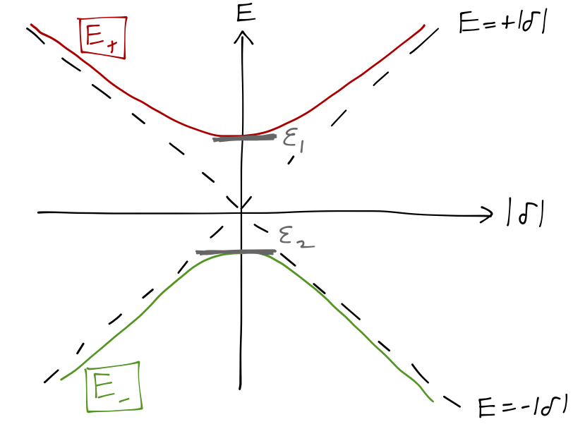
This is an example of a phenomenon known as avoided level crossing. The two curves for \( \epsilon_1 \) and \( \epsilon_2 \) can never cross in this system, except in the special case where the splitting \( \epsilon = 0 \), where the eigenvalues become degenerate at \( \delta = 0 \). When the energies are degenerate, the system is in a state of enhanced symmetry; including either \( \epsilon \) or \( \delta \) breaks the symmetry, and there can be no level crossing. This is actually quite a general result, but this is just a preview; we can't elaborate on the general no-crossing theorem until we study perturbation theory.
Next time: back to time evolution.