Example: Larmor precession
Now that we understand the energy eigenstates in the generalized two-state system, let's see what happens to it under time evolution. Having worked out the general case, we will return now to the specific example of an electron in an external magnetic field, with Hamiltonian
\[ \begin{aligned} \hat{H} = -\hat{\vec{\mu}} \cdot \vec{B} = \frac{e}{mc} \hat{\vec{S}} \cdot \vec{B}. \end{aligned} \]
As the hats remind us, the magnetic field is a classical field which exists in the background, so it's not an operator, just an ordinary vector. In fact, in the usual \( \hat{S_z} \) basis we know that the spin operators are proportional to the Pauli matrices \( \vec{\sigma} \), and so we can expand out the dot product as
\[ \begin{aligned} \hat{\vec{S}} \cdot \vec{B} = \frac{\hbar}{2} \hat{\vec{\sigma}} \cdot \vec{B} = \frac{\hbar}{2} \left( \begin{array}{cc} B_z & B_x - iB_y \\ B_x + iB_y & -B_z \end{array} \right). \end{aligned} \]
It's convenient to define the quantity
\[ \begin{aligned} \omega = \frac{e|B|}{mc} \end{aligned} \]
in which case we simply have
\[ \begin{aligned} \hat{H} = \frac{\hbar \omega}{2} (\hat{\vec{\sigma}} \cdot \vec{n}), \end{aligned} \]
where \( \vec{n} \) is a unit vector pointing in the direction of the applied magnetic field. The angular frequency \( \omega \) is known as the Larmor frequency.
(A word of warning: I'm following Sakurai and using "Gaussian" or "cgs" units, which includes some extra factors of \( c \) in the definitions of electromagnetic fields. See appendix A for how to convert between Gaussian and SI units. If you try to plug in an SI magnetic field above you will get a wave number and not a frequency, so at least you'll know something is wrong!)
In general, the Hamiltonian will not commute with any of the spin operators, since it is a combination of all three. However, since we're studying the spin-1/2 system in complete isolation, there's nothing stopping us from calling the magnetic field direction \( z \). Then we can see that \( [\hat{H}, \hat{S_z}] = 0 \), and our Hamiltonian becomes
\[ \begin{aligned} \hat{H} = \frac{\hbar \omega}{2} \left( \begin{array}{cc} 1 & 0 \\ 0 & -1 \end{array} \right) \end{aligned} \]
which is already diagonal, with eigenvalues \( E_{\pm} = \pm \hbar \omega/2 \). So if at \( t=0 \) our system is in the state
\[ \begin{aligned} \ket{\psi(0)} = \alpha \ket{+} + \beta \ket{-}, \end{aligned} \]
then at time \( t \) we will find the state
\[ \begin{aligned} \ket{\psi(t)} = \alpha e^{-i\omega t/2} \ket{+} + \beta e^{+i\omega t/2} \ket{-}. \end{aligned} \]
As we've noted, for an operator which commutes with \( \hat{H} \) its eigenstates will remain eigenstates for all time, and indeed we find that if \( \ket{\psi(0)} = \ket{+} \), then at any \( t \) the probability of measuring \( \ket{+} \) is
\[ \begin{aligned} P(+) = |\sprod{\psi(t)}{+}|^2 = |\bra{+} e^{i\omega t/2} \ket{+}|^2 = 1. \end{aligned} \]
A more interesting example is the initial state
\[ \begin{aligned} \ket{\psi(0)} = \frac{1}{\sqrt{2}} (\ket{+} + \ket{-}), \end{aligned} \]
which you'll recognize as the spin-up eigenket in the \( x \) direction. This state will not remain stationary; in particular, we can calculate the probability of measuring spin-up in \( \hat{S_x} \) at time \( t \) as
\[ \begin{aligned} P(S_x = +\hbar/2) = |\sprod{S_{x,+}}{\psi(t)}|^2 = \left| \frac{1}{\sqrt{2}} \left( \bra{+} + \bra{-} \right) \frac{1}{\sqrt{2}} \left( e^{-i\omega t/2} \ket{+} + e^{i\omega t /2} \ket{-} \right) \right|^2 \\ = \frac{1}{4} \left| e^{-i\omega t/2} + e^{i\omega t /2} \right|^2 \\ = \cos^2 \frac{\omega t}{2}. \end{aligned} \]
We can go through the exercise of finding the spin-down probability the same way, but of course the total probability has to be 1, so we know already that it must be \( P(S_x = -\hbar/2) = \sin^2 (\omega t / 2) \). Knowing the probability of being in either eigenstate lets us immediately construct the average value \( \ev{\hat{S_x}} \):
\[ \begin{aligned} \ev{\hat{S_x}} = \frac{\hbar}{2} \cos^2 \frac{\omega t}{2} + \left(\frac{-\hbar}{2}\right) \sin^2 \frac{\omega t}{2} \\ = \frac{\hbar}{2} \cos \omega t \end{aligned} \]
So indeed, if we carry out an experiment keeping track of the average spin in the \( x \) direction under an applied magnetic field in the \( z \) direction, we will find oscillation at exactly the Larmor frequency. In fact, we can perform a similar calculation to find that in this situation,
\[ \begin{aligned} \ev{\hat{S_y}} = \frac{\hbar}{2} \sin \omega t, \\ \ev{\hat{S_z}} = 0. \end{aligned} \]
The applied \( z \)-direction magnetic field causes the spin to rotate, or precess, in the \( xy \) plane; this particular example is known as Larmor precession. This is a very important effect; I've glossed over the point that the Larmor precession frequency is more generally defined as
\[ \begin{aligned} \omega = \frac{eg|B|}{2mc}, \end{aligned} \]
where the quantity \( g \) is an intrinsic property of the charged object, relating angular momentum to the magnetic moment. For a classical spinning charged sphere, \( g=1 \); for the electron, quantum effects lead to \( g=2 \).
In fact, \( g \) is not exactly two for the electron; quantum electrodynamics, the quantum field theory which describes the electromagnetic force, predicts small corrections as a power series in the fine-structure constant \( \alpha \approx 1/137 \). Experiments to measure the Larmor precession of electrons and theoretical calculations of this power series have been carried out to extraordinary precision, and the agreement between the two is now at a level below 1 part per trillion.
We've been doing a lot of theory, so let's talk briefly about experimental determination of the muon \( (g-2) \). (This is a more direct application of what we've just done than electron \( (g-2) \) experiments, which tend to exploit atomic physics.) The Larmor frequency \( \omega \) looks a lot like a familiar classical expression, which is the cyclotron frequency: a classical charge of magnitude \( e \) will undergo circular motion in a transverse magnetic field with angular frequency
\[ \begin{aligned} \omega_c = \frac{e|B|}{mc} \end{aligned} \]
This suggests a straightforward way to set up an experiment: we inject a beam of muons into a circular storage ring with magnetic field applied in the \( \hat{z} \) direction. The muon is unstable and will decay into an electron (plus neutrinos), and the direction of the outgoing electron turns out to be correlated with the direction of the muon's spin, so we can measure the spin direction by looking for electrons coming out.
Now, if \( g \) is exactly 2 for the muon, then if we put a detector at a fixed point on our storage ring, the spin will precess at precisely the same rate as the motion around the ring, which means that we should never see any variation in the muon's spin direction. If there is an anomalous contribution to \( (g-2) \), then we'll see it as a modulated signal, i.e. we expect an anomalous precession frequency
\[ \begin{aligned} \omega_a = \frac{(g-2)e|B|}{2mc}. \end{aligned} \]
Here's what the E821 experiment done at Brookhaven National Laboratory saw:
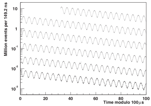
By eye, the oscillation period is about 5 microseconds, which translates to \( (g-2)/2 \sim 0.001 \). Of course, this is just a summary plot, the real experimental measurement is much more precise:
\[ \begin{aligned} \frac{g_\mu - 2}{2} = 0.0011659208(5)(3). \end{aligned} \]
I've ignored all kinds of important details here, of course, not least of which is relativistic effects since the muons have to be moving pretty fast to make the experiment work! But the basic idea here is very simple. The experiment itself is a masterful piece of precision physics, and if you're interested I invite you to look at the final report of the E821 experiment to see all the details.
The Standard Model of particle physics predicts a value of the muon \( (g-2) \) which is very close to the number given above, but actually around 4 standard deviations different based on our best estimates of the theoretical uncertainty - perhaps a tantalizing hint of new physics around the corner? A new experiment at Fermilab will seek to answer the question on the experimental side soon!
Exponentiating the two-state Hamiltonian
The previous example exploited the fact that time evolution acts simply on eigenstates of the Hamiltonian, which were also eigenstates of the \( \hat{S}_z \) operator. However, more generally we might be interested in the case where the Hamiltonian is not simply proportional to \( \hat{S}_z \). If we allow the magnetic field to point in any direction, then we find the Hamiltonian
\[ \begin{aligned} \hat{H} = \frac{\hbar \omega}{2} \hat{\vec{\sigma}} \cdot \vec{n}, \end{aligned} \]
where \( \vec{n} = \vec{B} / |\vec{B}| \) is a unit vector in the direction of the applied magnetic field. (If this is the entire Hamiltonian, then we're just making life harder for ourselves by not rotating our coordinates to make \( \vec{n} = \hat{z} \)! But there are plenty of systems that have this interaction as one of many.)
Recall that earlier we wrote down a formal expression for the time-evolution operator when \( \hat{H} \) itself is time-independent, namely
\[ \begin{aligned} \hat{U}(t) = e^{-i\hat{H} t/\hbar} = e^{-i \omega t \hat{\vec{\sigma}} \cdot \vec{n}/2}. \end{aligned} \]
We know that this exponential can be rewritten as a power series,
\[ \begin{aligned} e^{-i\omega t \hat{\vec{\sigma}} \cdot \vec{n}/2} = \hat{1} - \frac{i \omega t}{2} (\hat{\vec{\sigma}} \cdot \vec{n}) + \frac{1}{2} \left(\frac{i \omega t}{2}\right)^2 (\hat{\vec{\sigma}} \cdot \vec{n})^2 + ... \end{aligned} \]
Taking powers of \( (\hat{\vec{\sigma}} \cdot \vec{n}) \) isn't as easy as it looks, since we know the three Pauli matrices don't commute with each other. However, we can show that the product of two Pauli matrices satisfies the identity
\[ \begin{aligned} \hat{\sigma}_i \hat{\sigma}_j = i \epsilon_{ijk} \hat{\sigma}_k + \hat{1} \delta_{ij}, \end{aligned} \]
and thus
\[ \begin{aligned} (\hat{\vec{\sigma}} \cdot \vec{n})^2 = \hat{\sigma}_i n_i \hat{\sigma}_j n_j \\ = \left( i \epsilon_{ijk} \hat{\sigma}_k + \hat{1} \delta_{ij} \right) n_i n_j. \end{aligned} \]
(Note that here I am using the Einstein summation convention, that when you see repeated indices they are implicitly summed over. If it's ever unclear in a particular situation I will write explicit sums.)
Anyway, since \( \vec{n} \) is a unit vector pointing in some direction, we know that \( \epsilon_{ijk} n_i nj = \vec{n} \times \vec{n} = 0 \), and \( \delta{ij} n_i n_j = \vec{n} \cdot \vec{n} = 1 \). So \( (\hat{\vec{\sigma}} \cdot \vec{n})^2 = \hat{1} \), which means that \( (\hat{\vec{\sigma}} \cdot \vec{n})^3 = \hat{\vec{\sigma}} \cdot \vec{n} \), and so forth. This immediately lets us write our infinite sum of matrix products as a pair of infinite sums multiplied by known matrices:
\[ \begin{aligned} e^{-i\omega t \hat{\vec{\sigma}} \cdot \vec{n}/2} = \sum_{k=0}^\infty \frac{1}{k!} \left[ \left(\frac{i \omega t}{2}\right) \hat{\vec{\sigma}} \cdot \vec{n}\right]^k \\ = \sum_{k=0}^\infty \left[ \frac{1}{(2k)!} (i \omega t)^{2k} \hat{1} + \frac{1}{(2k+1)!} (i \omega t)^{2k+1} (\hat{\vec{\sigma}} \cdot \vec{n}) \right] \\ = \hat{1} \cos \frac{\omega t}{2} - i (\hat{\vec{\sigma}} \cdot \vec{n}) \sin \frac{\omega t}{2}. \end{aligned} \]
Writing it out in matrix form,
\[ \begin{aligned} \hat{U}(t) = \left( \begin{array}{cc} \cos \omega t/2 - i n_z \sin \omega t/2 & (-i n_x - n_y) \sin \omega t/2 \\ (-i n_x + n_y) \sin \omega t/2 & \cos \omega t/2 + i n_z \sin \omega t/2 \end{array} \right). \end{aligned} \]
I leave it as an exercise to verify that this is (as expected) a unitary matrix, i.e. \( \hat{U}^\dagger \hat{U} = \hat{1} \), and that setting \( n_z = 1 \) recovers the time evolution we found in the Larmor precession example.
Aside: solving without exponentiation
It's instructive to see another way to calculate the same matrix, which is easier to work with in cases where summing the power series as we did above is hard. Remember that we can rewrite the time evolution operator by summing over energy eigenstates,
\[ \begin{aligned} \hat{U}(t) = e^{- i\hat{H}t / \hbar} = \sum_{i} \sum_j \ket{E_i} \bra{E_i} e^{-i\hat{H} t/\hbar} \ket{E_j} \bra{E_j} \\ = \sum_i \ket{E_i} e^{-i \hat{E_i} t/\hbar} \bra{E_i}. \end{aligned} \]
So to find the evolution operator, we just need to compute the eigenvalues and eigenvectors of \( \hat{H} \), which in matrix form looks like
\[ \begin{aligned} \hat{H} = \frac{\hbar \omega}{2} \left( \begin{array}{cc} n_z & n_x - in_y \\ n_x + in_y & -n_z \end{array} \right). \end{aligned} \]
We diagonalized this matrix last time; here we identify the energy splitting \( \epsilon = \hbar \omega n_z/2 \) and the off-diagonal term \( \delta = \hbar \omega (n_x - in_y) / 2 \). The average energy is 0, so that the energy eigenvalues are
\[ \begin{aligned} E_{\pm} = \pm \sqrt{\epsilon^2 + |\delta|^2} = \pm \sqrt{ (\hbar \omega / 2)^2} \sqrt{n_z^2 + n_x^2 + n_y^2} = \pm \hbar \omega/2. \end{aligned} \]
The mixing angle which determines the eigenstates is
\[ \begin{aligned} \tan 2\alpha = \frac{\epsilon}{|\delta|} = \frac{n_z}{\sqrt{n_x^2 + n_y^2}} \end{aligned} \]
and the phase \( \phi \) is given by the expression
\[ \begin{aligned} e^{i\phi} = \frac{\delta^\star}{|\delta|} = \frac{n_x + in_y}{\sqrt{n_x^2 + n_y^2}} \end{aligned} \]
These are, in fact, exactly the spherical angles defining the unit vector \( \vec{n} \) itself! The only oddity is that the mixing angle \( \alpha \) is half of the coordinate-space angle \( \theta \). So the eigenstates are, referring back to our previous work,
\[ \begin{aligned} \ket{+} = \left( \begin{array}{c} \cos (\theta/2) \\ \sin (\theta/2) e^{i \phi} \end{array} \right) \\ \ket{-} = \left( \begin{array}{c} -\sin (\theta/2) e^{-i\phi} \\ \cos (\theta/2) \end{array} \right) \end{aligned} \]
giving the outer products
\[ \begin{aligned} \hat{U}(t) = e^{-i \omega t/ 2} \ket{+} \bra{+} + e^{i \omega t /2} \ket{-} \bra{-} \\ = \left( \begin{array}{cc} \cos^2 (\theta/2) e^{-i\omega t/2} + \sin^2 (\theta/2) e^{i \omega t/2} & \cos (\theta/2) \sin (\theta/2) e^{-i\phi} (e^{-i \omega t/2} - e^{i \omega t /2}) \\ \cos (\theta/2) \sin (\theta/2) e^{i\phi} (e^{-i \omega t/2} - e^{i \omega t/2}) & \sin^2 (\theta/2) e^{-i\omega t/2} + \cos^2 (\theta/2) e^{i \omega t/2} \end{array} \right) \\ = \left( \begin{array}{cc} \cos (\omega t/2) - i \cos \theta \sin (\omega t/2) & -i\sin (\omega t/2) \sin \theta e^{-i \phi} \\ -i\sin(\omega t/2) \sin \theta e^{i\phi} & \cos (\omega t /2) + i \cos \theta \sin(\omega t/2) \end{array} \right) \end{aligned} \]
recovering our result above, in a slightly different notation.
Example: magnetic resonance
As a lead-in to our next topic, let's look at another situation which is very hard to deal with in general, but tractable for the two-state system; explicit time variation in the Hamiltonian. The physical effect that we will be studying here is known as magnetic resonance, and is one of the more important applications of the two-state system.
(Note: beware factors of 2 in the definitions of frequencies if you look up this derivation elsewhere!)
Let's apply an external magnetic field which has a large, constant component \( B \) in the \( z \) direction, and a small component which rotates around the \( xy \) plane with angular frequency \( \nu \):
\[ \begin{aligned} \vec{B} = (b \cos \nu t, b \sin \nu t, B). \end{aligned} \]
This is just a specific choice of an external magnetic field, so we can write the Hamiltonian like we did in the previous example,
\[ \begin{aligned} \hat{H} = \frac{\hbar \omega}{2} \hat{\sigma}_z + \frac{\hbar \Omega_0}{2} \left( \hat{\sigma}_x \cos (\nu t) + \hat{\sigma}_y \sin (\nu t) \right) = \frac{\hbar}{2} \left( \begin{array}{cc} \omega & \Omega_0 e^{-i\nu t} \\ \Omega_0 e^{i \nu t} & -\omega \end{array} \right) \end{aligned} \]
where we've now defined two angular frequencies
\[ \begin{aligned} \omega = \frac{eB}{mc}, \\ \Omega_0 = \frac{eb}{mc}. \end{aligned} \]
This time, we'll apply the Schrödinger equation directly; since this is a two-state system, we end up with a pair of coupled differential equations. If we define
\[ \begin{aligned} \ket{\psi(t)} = \left( \begin{array}{c} a_+(t) \\ a_-(t) \end{array} \right) \end{aligned} \]
then applying the Hamiltonian, we find
\[ \begin{aligned} i \hbar \frac{d}{dt} \ket{\psi(t)} = \hat{H} \ket{\psi(t)} \\ \begin{cases} 2i \frac{da_+}{dt} &= \omega a_+ + \Omega_0 e^{-i\nu t} a_- \\ 2i \frac{da_-}{dt} &= \Omega_0 e^{i\nu t} a_+ - \omega a_-. \end{cases} \end{aligned} \]
We can solve this coupled system by ansatz (physics jargon for a clever guess). Noticing the complex exponential time dependence, if we assume the same is true for the wavefunction solution, i.e.
\[ \begin{aligned} a_{\pm} = A_{\pm} e^{-i \lambda_{\pm} t}, \end{aligned} \]
then in matrix form, we arrive at the equation
\[ \begin{aligned} \left( \begin{array}{cc} 2\lambda_+ - \omega & -\Omega_0 e^{-i(\nu -\lambda_+ + \lambda_-)t} \\ -\Omega_0 e^{i(\nu - \lambda_+ + \lambda_-)t} & 2 \lambda_- + \omega \end{array} \right) \left( \begin{array}{c} A_+ \\ A_- \end{array} \right) = 0. \end{aligned} \]
Now we see that the time dependence is entirely removed if we choose \( \lambda_+ = \lambda_- + \nu \). That just leaves us with the simple system
\[ \begin{aligned} \left( \begin{array}{cc} 2\lambda_- + 2\nu - \omega & -\Omega_0 \\ -\Omega_0 & 2\lambda_- + \omega \end{array} \right) \left( \begin{array}{c} A_+ \\ A_- \end{array} \right) = 0. \end{aligned} \]
Setting the determinant equal to zero gives us the condition for a solution to exist, which is
\[ \begin{aligned} \lambda_- = \frac{-\nu}{2} \pm \Omega, \\ \Omega = \sqrt{\Omega_0^2 + (\nu - \omega)^2}. \end{aligned} \]
The most general solution is a linear combination of the two possibilities, e.g.
\[ \begin{aligned} a_-(t) = A_-^{(1)} e^{-i(\Omega - \nu/2)t} + A_-^{(2)} e^{-i(-\Omega-\nu/2)t}. \end{aligned} \]
We can't proceed without specifying a boundary condition, here the state of the system at \( t=0 \) (the second constraint is provided by the overall normalization of the physical state.) For example, let's suppose that at \( t=0 \) our electron has spin up,
\[ \begin{aligned} \ket{\psi(0)} = \left( \begin{array}{c} 1 \\ 0 \end{array} \right). \end{aligned} \]
Then \( a_-(0) = 0 \), which requires us to take \( A_-^{(1)} = A_-^{(2)} \), and thus
\[ \begin{aligned} a_-(t) = A e^{i\nu t/2} \sin (t \Omega). \end{aligned} \]
Returning to the differential equations and evaluating one at \( t=0 \), we find
\[ \begin{aligned} i \frac{da_-(0)}{dt} = \Omega_0 a_+(0) - \omega a_-(0) \\ A \Omega = \Omega_0 \end{aligned} \]
where I've used \( a_+(0) = 1 \) and \( a_-(0) = 0 \). Thus, our solution is
\[ \begin{aligned} a_-(t) = \frac{\Omega_0}{\Omega} \sin (t \Omega) e^{i \nu t/2}. \end{aligned} \]
The probability that our initially spin-up electron flips to spin-down at time \( t \) is therefore
\[ \begin{aligned} P(-) = |a_-(t)|^2 = \frac{\Omega_0^2}{\Omega^2} \sin^2 (t \Omega). \end{aligned} \]
So the probability oscillates sinusoidally, but with a maximum given by
\[ \begin{aligned} \frac{\Omega_0^2}{\Omega^2} = \frac{\Omega_0^2}{\Omega_0^2 + (\omega - \nu)^2} \end{aligned} \]
If the applied field is strong, then this probability goes to 1 and \( \Omega \rightarrow \Omega_0 \). However, the more interesting case is when the applied field and therefore \( \Omega_0 \) is small. Then the probability amplitude exhibits resonance; it will be sharply peaked for \( \nu \approx \omega \). In fact, the functional form above for \( \Omega_0^2 / \Omega^2 \) is an example of a Lorentzian or Cauchy distribution. Its maximum will always occur around \( \nu \approx \omega \), and will be more sharply peaked as the strength of the rotating field \( b \) becomes small.
Magnetic resonance provides a powerful experimental tool for studying the properties of particles which carry spin; set up properly, we can learn \( \omega \) (and therefore, in our simple example, the charge and mass of the spinning particle) just by varying the driving frequency \( \nu \) and watching the response.