Last time, we ended on the observation that in the Heisenberg picture, the eigenkets of an operator must evolve in time: this is evident from the eigenvalue equation
\[ \begin{aligned} \hat{A}{}^{(H)}(t) \ket{a(t)} = a \ket{a(t)}, \end{aligned} \]
and we found the explicit time dependence of the eigenkets to be
\[ \begin{aligned} \ket{a(t)} = \hat{U}{}^\dagger (t) \ket{a(0)}, \end{aligned} \]
precisely the opposite of how state vectors evolve in the Schrödinger picture.
This starts to get confusing if we are using an operator to define a basis, which we often do in quantum mechanics! Suppose we have a state vector that we have expanded out in the eigenbasis of \( \hat{A} \) at time zero:
\[ \begin{aligned} \ket{\psi(0)} = \sum_{a} c_\psi(a) \ket{a} \end{aligned} \]
where \( c_\psi(a) = \sprod{a}{\psi} \). In the Schrödinger picture, the basis states are fixed, and so to include time evolution we just have to make the coefficients \( c_\psi(a) \) time-dependent:
\[ \begin{aligned} \ket{\psi(t)}^{(S)} = \sum_{a} c_\psi^{(S)}(a,t) \ket{a} \end{aligned} \]
which is straightforward. In the Heisenberg picture, our basis changes but the state vector is fixed - which means the coefficients of the expansion are still time-dependent:
\[ \begin{aligned} \ket{\psi}^{(H)} = \sum_{a} c_\psi^{(H)}(a,t) \ket{a(t)} \end{aligned} \]
in such a way that the time dependence must cancel between the \( c_\psi^{(H)} \) and the \( \ket{a(t)} \)! If this seems completely bizarre, an analogy back to ordinary vector spaces might help here.
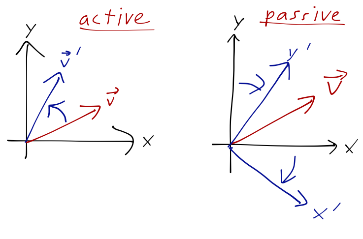
We can think of a unitary transformation like the time-evolution operator as a rotation acting on the kets (vectors) in our Hilbert space. In Schrödinger picture, time evolution is an active transformation; we begin with a state vector at \( t=0 \), and the rotation maps it to a new state vector. Heisenberg picture, on the other hand, is a passive transformation: the state vector is kept fixed and we rotate the coordinate system (the eigenbasis kets) around in the opposite direction. The end result is the same.
Just to drive the point home, if we ask a good, physical question, like "what is the probability amplitude for the system which exists in state \( \ket{\psi} \) at \( t=0 \) to be observed in an eigenstate \( \ket{b} \) of operator \( \hat{B} \) at time \( t \)", then the answer in the Schrödinger picture is
\[ \begin{aligned} p(b,t) = \sprod{b}{\psi(t)} = \bra{b} \left( e^{-i\hat{H} t/\hbar} \ket{\psi(0)} \right), \end{aligned} \]
while in the Heisenberg picture, it is the same thing with a different association:
\[ \begin{aligned} p(b,t) = \sprod{b(t)}{\psi} = \left( \bra{b} e^{-i\hat{H} t/\hbar} \right) \ket{\psi(0)}. \end{aligned} \]
Time evolution and the SHO
Back to the simple harmonic oscillator:
\[ \begin{aligned} \hat{H} = \frac{\hat{p}{}^2}{2m} + \frac{1}{2} m \omega^2 \hat{x}{}^2 \end{aligned} \]
Let's work in the Heisenberg picture. The equations of motion for the position and momentum operators are
\[ \begin{aligned} \frac{d\hat{p}}{dt} = \frac{1}{i\hbar} [\hat{p}, \hat{H}] = - m\omega^2 \hat{x} \\ \frac{d\hat{x}}{dt} = \frac{1}{i\hbar} [\hat{x}, \hat{H}] = \frac{\hat{p}}{m}, \end{aligned} \]
mimicking the classical equations of motion. On to the ladder operators; we could compute their time evolution directly, but since we did it for \( \hat{p} \) and \( \hat{x} \) already let's just use the change of variables,
\[ \begin{aligned} \frac{d\hat{a}}{dt} = \sqrt{\frac{m\omega}{2\hbar}} \left( \frac{\hat{p}}{m} + \frac{i}{m \omega} (-m \omega^2 \hat{x}) \right) \\ = -i \omega \hat{a}, \frac{d\hat{a}{}^\dagger}{dt} = i \omega \hat{a}{}^\dagger. \end{aligned} \]
These are nice and easy to solve:
\[ \begin{aligned} \hat{a}(t) = e^{-i\omega t} \hat{a}(0) \\ \hat{a}{}^\dagger (t) = e^{i \omega t} \hat{a}{}^\dagger(0). \end{aligned} \]
It's easy to see that the number operator \( \hat{N} = \hat{a}^\dagger \hat{a} \) is time-independent, which it should be since it commutes with \( \hat{H} \). Working backwards with our definitions of \( \hat{x} \) and \( \hat{p} \) in terms of the ladder operators, it's easy to show that
\[ \begin{aligned} \hat{x}(t) = \hat{x}(0) \cos \omega t + \frac{\hat{p}(0)}{m\omega} \sin \omega t \\ \hat{p}(t) = - m \omega \hat{x}(0) \sin \omega t + \hat{p}(0) \cos \omega t \end{aligned} \]
So the quantum observables oscillate at frequency \( \omega \), just like their classical counterparts.
There's another way to derive these results which is instructive. Instead of using the ladder operators, we can just attempt to directly evaluate the time evolution operator, i.e.
\[ \begin{aligned} \hat{x}(t) = e^{i\hat{H} t/\hbar} \hat{x}(0) e^{-i \hat{H} t/\hbar}. \end{aligned} \]
and similarly for \( \hat{p}(t) \). There is a very nice formula for operators sandwiched between exponentials like this, called the Baker-Hausdorff lemma: if \( \hat{A} \) and \( \hat{G} \) are Hermitian operators, then
\[ \begin{aligned} e^{i\hat{G} \lambda} \hat{A} e^{-i\hat{G} \lambda} = \hat{A} + i \lambda [\hat{G}, \hat{A}] - \frac{\lambda^2}{2} [\hat{G}, [\hat{G}, \hat{A}] ] + ... \\ \ + \left( \frac{i^n \lambda^n}{n!} \right) [\hat{G}, [\hat{G}, [\hat{G}, ...[\hat{G}, \hat{A}] ] ]...] + ... \end{aligned} \]
The commutation relations of the SHO Hamiltonian at \( t=0 \) happen to give rise to a repeating structure:
\[ \begin{aligned} [\hat{H}, \hat{x}(0)] = -\frac{i \hbar}{m} \hat{p}(0) \\ [\hat{H}, \hat{p}(0)] = i \hbar m \omega^2 \hat{x}(0). \end{aligned} \]
Similar to our previous example with the Pauli matrices, these relations let us split the infinite Baker-Hausdorff series into a pair of power series in ordinary numbers, multiplying the two operators \( \hat{x}(0) \) and \( \hat{p}(0) \). You should be able to see that the two power series are exactly the trigonometric functions, and so
\[ \begin{aligned} e^{i\hat{H} t/\hbar} \hat{x}(0) e^{-i\hat{H} t/\hbar} = \hat{x}(0) \cos \omega t + \frac{\hat{p}(0)}{m \omega} \sin \omega t, \end{aligned} \]
exactly as we found above (and the same setup will work for \( \hat{p}(t) \), obviously.)
If we take expectation values, does the quantum harmonic oscillator behave just like the classical counterpart, i.e. with \( \ev{\hat{x}} \propto \sin \omega t \) and similar for \( \ev{\hat{p}} \)? Well, yes and no. In fact, if we take our state vector to be a pure energy eigenstate \( \ket{\psi} = \ket{n} \), then we find that both expectation values are zero at \( t=0 \):
\[ \begin{aligned} \ev{\hat{x}(0)} = \ev{\hat{p}(0)} = 0 \end{aligned} \]
In fact, it's easy to see in either picture that the expectation values are zero for all time; in Schrödinger picture the energy eigenstates don't evolve except for a phase, and in Heisenberg picture we can think of the evolution cancelling between the basis kets and the operators (try not to get confused by the state ket being equal to a basis ket at \( t=0 \) here.) This doesn't contradict Ehrenfest's theorem, since we find that
\[ \begin{aligned} m \frac{d^2 \ev{\hat{x}}}{dt^2} = \ev{\nabla V(x)} = \ev{m\omega^2 \hat{x}} = 0. \end{aligned} \]
It is possible to construct a quantum state which will behave (on average) like a classical particle in the oscillator; in fact, these states are the coherent states, eigenstates of the lowering operator. You'll study coherent states a bit on this week's homework.
Interaction picture
The difference between Schrödinger picture and Heisenberg picture, as we have seen, is just a matter of organization: whether we prefer to keep the time evolution operator \( \hat{U} \) with the state kets or with the basis kets. There is another, more complicated possibility, which is that we can divide up the time evolution and assign part of it to both.
Why would we ever do such a thing? The best reason is to work in a specific third picture, called the interaction picture. Here, we start by dividing up the Hamiltonian into a piece which is time-independent and relatively simple, and "everything else":
\[ \begin{aligned} \hat{H} = \hat{H}_0 + \hat{V} \end{aligned} \]
The interaction-picture states are defined from the Schrödinger picture states as
\[ \begin{aligned} \ket{\psi(t)}_I = e^{i \hat{H}_0 t/\hbar} \ket{\psi(t)}_S \end{aligned} \]
(note the minus sign with respect to the Schrödinger equation solution!) which means that to keep matrix elements invariant, the operators must be defined to be
\[ \begin{aligned} \hat{O}{}^{(I)}(t) = e^{i\hat{H}_0 t/\hbar} \hat{O} e^{-i\hat{H}_0 t/\hbar} \end{aligned} \]
How do the interaction-picture states evolve in time? We can apply the Schrödinger equation to the original states:
\[ \begin{aligned} i \hbar \frac{\partial}{\partial t} \ket{\psi(t)}_I = -\hat{H}_0 e^{i\hat{H}_0 t/\hbar} \ket{\psi(t)}_S + e^{i\hat{H}_0 t/\hbar} \left( i \hbar \frac{\partial}{\partial t} \ket{\psi(t)}_S \right) \\ = -\hat{H}_0 \ket{\psi(t)}_I + e^{i \hat{H}_0 t/\hbar} (\hat{H}_0 + \hat{V}) \ket{\psi(t)}_S \\ = - \hat{H}_0 \ket{\psi(t)}_I + (\hat{H}_0 + e^{i\hat{H}_0 t/\hbar} \hat{V} e^{-i\hat{H}_0 t/\hbar}) \ket{\psi(t)}_I \\ = \hat{V}{}^{(I)} \ket{\psi(t)}_I. \end{aligned} \]
So the interaction-picture states evolve according to the Schrödinger equation, but with the full Hamiltonian replaced with just the terms contained in \( \hat{V} \). Meanwhile, our definition of the operators above indicates that they evolve according to the Heisenberg equation, but with the other piece \( \hat{H}_0 \):
\[ \begin{aligned} \frac{d \hat{O}{}^{(I)}}{dt} = \frac{1}{i\hbar} [\hat{O}{}^{(I)}, \hat{H}_0] + \frac{\partial \hat{O}{}^{(I)}}{\partial t}. \end{aligned} \]
We won't see the interaction picture much more this semester, but it is extremely important, particularly for time-dependent perturbation theory, where all of the small time-dependent terms are gathered in \( \hat{V} \), separated out from the simple time-independent evolution dictated by \( \hat{H}_0 \). Being able to rely on a complete analytic solution for the spectrum of \( \hat{H}_0 \) is often an excellent starting point to understand the more complex system with \( \hat{V} \) included. In quantum field theory (fully relativistic QM), the interaction picture is used almost exclusively, separating out the simple propagation of free particles and their interactions, which are treated perturbatively.
Wave mechanics
Now that we've developed a lot of the tools, notation, and formalism behind quantum mechanics, I'd like to spend some time working through a number of explicit examples. We'll mostly focus on wave mechanics, that is to say the solution of the Schrödinger wave equation for the position-space wavefunction \( \psi(x) \). Also, we're not going to just be solving arbitrary problems; every example I pick is going to show off some new feature or calculational method that's interesting to know about. But I thought it would be a nice change of pace to do some more concrete calculations.
For all of its virtues, Sakurai is a bit light on examples, particularly in wave mechanics; I'll be drawing heavily on other resources here, mainly the books by Merzbacher and Cohen-Tannoudji. I'll try to show everything in a self-contained way in my own lecture notes, and some results are briefly collected in Appendix B of Sakurai.
Example 1: the potential step
As I said, we'll start with wave mechanics in one dimension. We have a single particle of mass \( m \), moving subject to the potential step
\[ \begin{aligned} V(x) = \begin{cases} V_0, & x \geq 0 \\ 0, & x < 0. \end{cases} \end{aligned} \]
Far away from the step at \( x=0 \), we simply have a free particle propagating in a constant potential energy \( V \). We have previously derived the time-dependent Schrödinger equation for a single particle: taking \( i\hbar \frac{\partial}{\partial t}\ket{\psi} = \hat{H} \ket{\psi} \) and substituting in the form of the Hamiltonian operator in position space, we found
\[ \begin{aligned} i \hbar \frac{\partial \psi(\vec{x}, t)}{\partial t} = -\frac{\hbar^2}{2m} \nabla^2 \psi(\vec{x}, t) + V(\vec{x}) \psi(\vec{x}, t) \end{aligned} \]
As we've seen, the energy eigenfunctions are guaranteed to evolve in time in a particularly simple way, just picking up a phase. Therefore in many situations it's useful to start instead with the eigenvalue equation \( \hat{H} \ket{\psi} = E \ket{\psi} \), which leads to the time-independent Schrödinger equation
\[ \begin{aligned} -\frac{\hbar^2}{2m} \nabla^2 \psi(\vec{x}, t) + (V(\vec{x}) - E) \psi(\vec{x}, t) = 0 \end{aligned} \]
Here we specialize to one-dimensional motion, so the equation becomes
\[ \begin{aligned} -\frac{\hbar^2}{2m} \psi''(x) + V(x) \psi(x) = E \psi(x). \end{aligned} \]
If \( V(x) = V \) is a constant, then the solutions to this simple differential equation are plane waves:
\[ \begin{aligned} \psi(x) = A e^{ikx} + B e^{-ikx} \end{aligned} \]
where the wave number is
\[ \begin{aligned} k = \sqrt{2m(E-V)}/\hbar. \end{aligned} \]
There are three interesting cases to consider here: \( E<0,\ E>V_0 \), and \( 0 \leq E \leq V_0 \). Let's consider \( E<0 \) first; classically this solution corresponds to negative kinetic energy, and is forbidden. In quantum mechanics, it is still forbidden. For \( E<0 \), we find that over all of space, the wave number \( k \) is imaginary, which means that the solutions are pure exponentials. But exponential functions aren't normalizable; there is no way to have a wavefunction with overall norm 1,
\[ \begin{aligned} \int_{-\infty}^{\infty} dx\ |\psi(x)|^2 = 1, \end{aligned} \]
with pure exponential solutions. In fact, a more general theorem can be proven from the Schrödinger equation: no solutions exist for \( E \) below the global minimum of the potential \( V(x) \).
Next, let's take \( E \) between \( 0 \) and \( V_0 \). For a classical particle, we would find reflection by the barrier; when the particle reaches \( x=0 \), the sign of its momentum will be flipped, conserving total energy. Quantum mechanically, we know the form of the solution on either side of the barrier:
\[ \begin{aligned} \psi(x) = \begin{cases} A e^{ikx} + Be^{-ikx} & (x < 0), \\ C e^{-\kappa x} & (x > 0) \end{cases} \end{aligned} \]
where now \( k = \sqrt{2mE} \) and \( \kappa = \sqrt{2m(V-E)}/\hbar \) is defined so we can just work with real numbers. In the quantum system a solution does exist even though locally \( E < V(x) \) for \( x>0 \); the negative-exponential solution is normalizable, since it doesn't extend to \( x = -\infty \) where it would blow up. The positive exponential \( e^{\kappa x} \) is still unphysical, so we discard it.
We can determine the coefficients \( A,B,C \) from the boundary condition, which is that our wavefunction \( \psi(x) \) and its derivative should both be continuous across the jump in the potential. It's easy to see why continuity is required, in fact for any potential function \( V(x) \) with a discontinuous jump at \( x_0 \). If we take the Schrödinger equation and integrate from \( x_0 - \epsilon \) to \( x_0 + \epsilon \) for some infinitesmal \( \epsilon \), then we find
\[ \begin{aligned} \psi'(x_0 + \epsilon) - \psi'(x_0 - \epsilon) = \int_{x_0 - \epsilon}^{x_0 + \epsilon} dx \frac{2m}{\hbar^2} \left[ V(x) - E \right] \psi(x) \end{aligned} \]
Since \( \psi(x) \) itself can't diverge (doing so would violate the probability interpretation), as long as \( V(x) \) is finite the integral will give a finite result that must vanish as \( \epsilon \rightarrow 0 \), and so the derivative \( \psi'(x) \) must be continuous across the potential jump. If the derivative is continuous, then so is \( \psi(x) \) itself.
Beware potentials containing delta functions! It's maybe obvious that if for something like an infinite barrier where \( V \) jumps to infinity discontinuously, the continuity of \( \psi(x) \) and its derivatives won't hold. In fact, in a region with infinite potential \( \psi(x) \) and all its derivatives must vanish, which gives us a different boundary condition. What if \( V(x) = a \delta(x-x_0) \)? Well, we see that
\[ \begin{aligned} \psi'(x_0 + \epsilon) - \psi'(x_0 - \epsilon) = \int_{x_0-\epsilon}^{x_0+\epsilon} dx \frac{2m}{\hbar^2} \left[ a \delta(x-x_0) - E \right] \psi(x) \\ = \frac{2ma}{\hbar^2} \psi(x_0) \end{aligned} \]
so we find (a very specific) discontinuity in the derivative of the wavefunction - and the wavefunction itself will be continuous across the delta function, since there's only a finite jump in the derivative of \( \psi(x) \).
Next time: more wave mechanics, and probability flux.