First, a remark about something that came up in last lecture. We derived the boundary conditions for matching solutions of the Schrödinger equation, and showed that for a finite \( V(x) \) the wavefunction \( \psi \) and its derivative \( \psi' \) must both be continuous. An important exception to this condition is the delta-function potential, in which case \( \psi' \) will have a specific discontinuity (but \( \psi \) is still continuous.) But what about the higher derivatives of \( \psi \)? Do we expect the wavefunction to be smooth in general, i.e. all derivatives to be continuous?
In fact, the answer is staring us in the face from the Schrödinger equation itself:
\[ \begin{aligned} -\frac{\hbar^2}{2m} \psi''(x) = [E-V(x)] \psi(x) \end{aligned} \]
Without any manipulation, we immediately see that the second derivative \( \psi'' \) is continuous as long as \( V(x) \) is continuous (and \( \psi(x) \) is continuous, but we already showed that must be true for finite \( V(x) \), so we can bootstrap our way up from there.)
We can then take a derivative and see that \( \psi''' \) is also continuous for any potential for which \( V'(x) \) is continuous, and so on. So a smooth \( V(x) \) will yield a smooth wavefunction, which is what I would have guessed. On the other hand, we are working with a counter-example right now: the step-function potential
\[ \begin{aligned} V(x) = \begin{cases} V_0, & x \geq 0 \\ 0, & x < 0. \end{cases} \end{aligned} \]
has a discontinuity at \( x=0 \), which means that \( \psi''(0) \) in this problem must have a discontinuity as well! In general, we could certainly do quantum mechanics using only smooth functions as long as we only work with smooth potentials, which are probably more realistic anyway. But things like step functions and delta functions are useful and simple approximations.
Last time, we ended considering the second of three interesting cases for energy eigenfunction solutions to the step-function potential, namely \( 0 < E \leq V_0 \). We argued that the general solution will take the form
\[ \begin{aligned} \psi(x) = \begin{cases} A e^{ikx} + Be^{-ikx} & (x < 0), \\ C e^{-\kappa x} & (x > 0). \end{cases} \end{aligned} \]
Now we apply our boundary conditions. Continuity of the wavefunction and its derivative at \( x=0 \) gives us two equations,
\[ \begin{aligned} A + B = C \\ ik(A-B) = -\kappa C. \end{aligned} \]
which we can solve for the ratios
\[ \begin{aligned} \frac{B}{A} = \frac{ik + \kappa}{ik - \kappa} \\ \frac{C}{A} = \frac{2ik}{ik - \kappa} = 1 + \frac{B}{A}. \end{aligned} \]
It's convenient to notice that \( B/A \) is a pure phase; if we multiply by its complex conjugate, we find \( |B/A| = 1 \), so we can write it as
\[ \begin{aligned} \frac{B}{A} = e^{i\alpha} \end{aligned} \]
for some real number \( \alpha \). If we plug these back into our general solution, we find the result
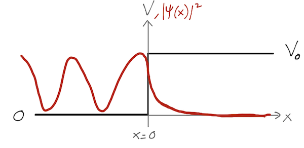
\[ \begin{aligned} \psi(x) = \begin{cases} 2A e^{i\alpha / 2} \cos \left( kx - \frac{\alpha}{2} \right) & (x<0) \\ 2A e^{i\alpha / 2} \cos \frac{\alpha}{2} e^{-\kappa x} & (x>0). \end{cases} \end{aligned} \]
Notice that in this case, it didn't matter what the energy \( E \) was; we could always find a solution which smoothly joined the exponential and plane-wave pieces of the wavefunction together.
How do we physically interpret this wavefunction? First, we should notice that unlike the classical case, the quantum particle has a non-zero probability \( |\psi(x)|^2 \) to be found in the classically forbidden region \( x>0 \); this probability is exponentially damped as \( x \) increases.
In the left-hand region, we notice that because \( B/A \) is a pure phase, we have \( |A|^2 \) = \( |B|^2 \). We can think of \( A \) and \( B \) as probability amplitudes associated with a right-moving and left-moving plane wave, respectively; the waves having equal (squared) amplitudes) therefore corresponds to total reflection. Indeed, if we construct a wave-packet solution out of solutions with \( 0 < E < V_0 \) and send it towards the barrier, it will end up propagating back to the left with the same amplitude as the incident packet, despite the fact that it may temporarily penetrate the barrier at \( x=0 \).
Probability density and flux, continuity equation
A brief aside: we've discussed the interpretation of \( |\psi(x)|^2 \) as a probability density. Now that we've introduced time evolution, this density can change in time as the wavefunction evolves, which leads us to the natural question: if we have a time-varying density, can we define a probability current? If we differentiate the probability density with respect to time, we find
\[ \begin{aligned} i\hbar \frac{\partial}{\partial t} (\psi^\star \psi) = i \hbar \frac{\partial \psi^\star}{\partial t} \psi + \psi^\star i\hbar \frac{\partial \psi}{\partial t} \\ = \psi^\star \left(-\frac{\hbar^2}{2m} \nabla^2 \psi + V \psi\right) - \left(-\frac{\hbar^2}{2m} \nabla^2 \psi^\star + V \psi^\star\right) \psi. \end{aligned} \]
The \( V \psi^\star \psi \) terms cancel out, and we can rewrite the other terms in a more symmetric way by moving one of the gradients outside, leading to
\[ \begin{aligned} \frac{\partial (\psi^\star \psi)}{\partial t} + \frac{\hbar}{2mi} \nabla \cdot \left[ \psi^\star \nabla \psi - (\nabla \psi^\star) \psi \right] = 0 \\ \frac{\partial \rho}{\partial t} + \nabla \cdot \vec{j} = 0. \end{aligned} \]
This is exactly the form of a continuity equation, which you'll recognize from e.g. classical electromagnetism; the rate of change of the local density is balanced by the divergence of the local current. We have identified the probability current or probability flux,
\[ \begin{aligned} \vec{j} = \frac{\hbar}{2mi} \left[ \psi^\star \nabla \psi - (\nabla \psi^\star) \psi \right] = \frac{\hbar}{m} \textrm{Im} (\psi^\star \nabla \psi). \end{aligned} \]
This is where the phase of the wavefunction, which cancels out in the local probability density, really has a physical effect. In fact, if we write explicitly
\[ \begin{aligned} \psi = \sqrt{\rho} e^{iS/\hbar} \end{aligned} \]
where both \( \rho \) and \( S \) are real (and the probability density \( \rho > 0 \)), then the flux becomes
\[ \begin{aligned} \textrm{Im} \left(\psi^\star \nabla \psi\right) = \textrm{Im} \left( \sqrt{\rho} \nabla (\sqrt{\rho}) + \frac{i}{\hbar} \rho \nabla S \right) \end{aligned} \]
and so
\[ \begin{aligned} \vec{j} = \frac{\rho \nabla S}{m}. \end{aligned} \]
So the gradient of the phase of the wavefunction encodes the strength of the probability current.
Notice that this derivation depended on the fact that \( V(x) \) is real, i.e. that the Hamiltonian operator was Hermitian. The conservation of probability implied by the continuity equation is only valid if \( \hat{H} \) is Hermitian. This doesn't mean that we should never consider a complex Hamiltonian; in fact, such an operator is useful for describing processes which are not conservative, e.g. decay or absorption of particles. We'll see an explicit example of that a bit later.
Back to our potential step example; what does the flow of probability look like in our solved example with \( 0 < E < V_0 \)? Well,
\[ \begin{aligned} \psi^\star \frac{d\psi}{dx} = \begin{cases} 4A^2 k \cos \left(kx - \frac{\alpha}{2}\right) \sin \left(kx - \frac{\alpha}{2} \right) & (x<0), \\ -4A^2 \kappa \cos \frac{\alpha}{2} e^{-\kappa x} & (x>0). \end{cases} \end{aligned} \]
This has zero imaginary part in both regions, so we conclude that \( \vec{j} = 0 \)! There is no net flow of probability in this solution. This is because we have solved explicitly for an energy eigenstate; we know that such a state only evolves in time by picking up a phase factor \( e^{iEt/\hbar} \), which cancels in the product \( \psi^\star \psi \). So the probability density \( \rho \) must be constant.
Now the last case: \( E > V_0 \). Classically, a particle incident from the left will continue moving to the right, but its velocity will decrease when it encounters the potential step. In the quantum system, we now have oscillating solutions on both sides of the step:
\[ \begin{aligned} \psi(x) = \begin{cases} A e^{ikx} + Be^{-ikx}, & (x<0) \\ C e^{ik'x} + De^{-ik'x}, & (x>0) \end{cases} \end{aligned} \]
where \( k=\sqrt{2mE}/\hbar \) as before, and \( k'=\sqrt{2m(E-V_0)}/\hbar \). Now our set of solutions is broader, since we have the same number of boundary conditions we will only be able to fix two out of four coefficients. Physically, the extra missing boundary condition has to do with how we think about the boundary at \( x = \pm \infty \). If we restore the time evolution, the two plane waves \( A \) and \( D \) represent incoming particles from infinity. In an experimental situation, we determine the relative strength of \( A \) and \( D \) based on the intensity at which we're sending in particles from the left and right.
If we want to interpret this as a single-particle solution, which is the most honest thing to do since we haven't really defined how to treat multiple particles mathematically yet, then it probably only makes sense to have either \( A \) or \( D \) non-zero, since our initial particle has to be sent in either from the left or from the right. Let's take \( D=0 \), so our incoming wave is \( A \). Then we find for the boundary conditions
\[ \begin{aligned} A + B = C \\ k(A-B) = k'C \end{aligned} \]
leading to the results
\[ \begin{aligned} \frac{B}{A} = \frac{k-k'}{k+k'} \\ \frac{C}{A} = \frac{2k}{k+k'}. \end{aligned} \]
This is no longer a pure phase, and correspondingly if we calculate the probability flux now, we no longer find zero:
\[ \begin{aligned} j = \begin{cases} \frac{\hbar k}{m} (|A|^2 - |B|^2), & (x<0) \\ \frac{\hbar k'}{m} |C|^2, & (x>0). \end{cases} \end{aligned} \]
(reducing to the previous \( j = 0 \) case for \( |A|^2 = |B|^2 \) as for the potential step.)
Now, we're still studying an energy eigenstate, which means that the gradient of the probability current is still zero everywhere, including at \( x=0 \); this means that the two constants above must be equal, leading to the requirement that
\[ \begin{aligned} \frac{|B|^2}{|A|^2} + \frac{k'}{k} \frac{|C|^2}{|A|^2} = 1. \end{aligned} \]
(This is not a new constraint: if we plug in \( B/A \) and \( C/A \) from above, it just reduces to \( 1=1 \). But it's another way to derive the relation between these ratios, which can be useful when it's harder to solve directly.)
The ratios \( B/A \) and \( C/A \) tell us the relative amplitude of the reflected and transmitted waves with respect to the incident wave, respectively. In particular, in analogy to optics we can define the reflection and transmission coefficients
\[ \begin{aligned} R = \frac{|B|^2}{|A|^2} = \frac{(k-k')^2}{(k+k')^2} \\ T = \frac{k'}{k} \frac{|C|^2}{|A|^2} = \frac{4kk'}{(k+k')^2}. \end{aligned} \]
Notice that the continuity equation tells us that \( R+T=1 \); this is the condition for conservation of probability. This is now obviously non-classical behavior; even though we are treating a single particle moving in a simple potential, it seems to "break apart" into reflected and transmitted pieces at the barrier. Reconciling this result with the fact that we see indivisible, identical particles like electrons strongly motivates particle-wave duality and the probability interpretation of the wave!
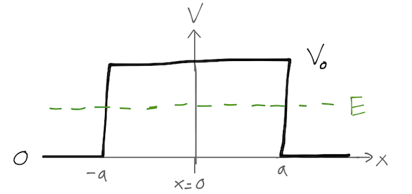
Example 2: The rectangular barrier
Now we can move on to a slightly more complicated system, the rectangular barrier potential:
\[ \begin{aligned} V(x) = \begin{cases} V_0, & |x| < a, \\ 0, & |x| > a. \end{cases} \end{aligned} \]
The most interesting case this time is \( E < V_0 \).
Once again the potential is piecewise constant, so we can start by writing down the solution to the Schrödinger equation, now in three parts:
\[ \begin{aligned} \psi(x) = \begin{cases} A e^{ikx} + Be^{-ikx}, & (x < -a); \\ C e^{-\kappa x} + De^{\kappa x}, & (-a < x < a); \\ F e^{ikx} + Ge^{-ikx}, & (x > a). \end{cases} \end{aligned} \]
with \( k \) and \( \kappa \) defined as above. Matching boundary conditions at the left boundary first, we have the pair of equations
\[ \begin{aligned} Ae^{-ika} + Be^{ika} = Ce^{\kappa a} + De^{-\kappa a} \\ Ae^{-ika} - Be^{ika} = \frac{i\kappa}{k} (Ce^{\kappa a} - De^{-\kappa a}). \end{aligned} \]
This is best re-expressed as a matrix equation:
\[ \begin{aligned} \left( \begin{array}{c} A \\ B \end{array} \right) = \frac{1}{2} \left( \begin{array}{cc} ze^{\kappa a + ika} & z^\star e^{-\kappa a + ika} \\ z^\star e^{\kappa a - ika} & z e^{-\kappa a - ika} \end{array} \right) \left( \begin{array}{c} C \\ D \end{array} \right) \end{aligned} \]
where \( z \equiv 1+i\kappa/k \). At the other barrier, we find a similar equation:
\[ \begin{aligned} \left( \begin{array}{c} C \\ D \end{array} \right) = \frac{1}{2} \left( \begin{array}{cc} z^\star e^{\kappa a + ika} & z e^{\kappa a - ika} \\ z e^{-\kappa a + ika} & z^\star e^{-\kappa a - ika} \end{array} \right) \left( \begin{array}{c} F \\ G \end{array} \right). \end{aligned} \]
This problem is a good model for situations where we scatter a free particle off of some target; in that context, we're not so interested in what happens inside the potential barrier, but more in what the relationship between the "input" and "output" free waves are. In other words, we'd really like to know the relationship between \( (A,B) \) and \( (F,G) \). The matrix equations make this simple to obtain, just by multiplying them together.
\[ \begin{aligned} \left( \begin{array}{c} A \\ B \end{array} \right) = \left( \begin{array}{cc} M_{11} & M_{12} \\ M_{21} & M_{22} \end{array} \right) \left( \begin{array}{c} F \\ G \end{array} \right). \end{aligned} \]
I won't write out the whole matrix because it's not particularly illuminating, but it's easy to derive from the above.
Next time: we finish this example, and more general scattering.