Last time, we started solving our second example, the rectangular barrier potential:
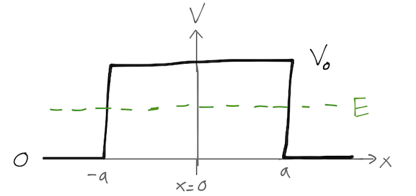
We wrote a piecewise solution with three pieces:
\[ \begin{aligned} \psi(x) = \begin{cases} A e^{ikx} + Be^{-ikx}, & (x < -a); \\ C e^{-\kappa x} + De^{\kappa x}, & (-a < x < a); \\ F e^{ikx} + Ge^{-ikx}, & (x > a). \end{cases} \end{aligned} \]
Matching the boundary conditions at both ends gives us some complicated algebra, but the important upshot is that we can write the result as a matrix \( M \):
\[ \begin{aligned} \left( \begin{array}{c} A \\ B \end{array} \right) = \left( \begin{array}{cc} M_{11} & M_{12} \\ M_{21} & M_{22} \end{array} \right) \left( \begin{array}{c} F \\ G \end{array} \right). \end{aligned} \]
This eliminates \( C \) and \( D \), which for most realistic experiments is just what we want: in the context of scattering, for example, we're more interested in how an incoming particle is related to an outgoing one than what happens in the middle of the potential barrier.
I'll note that there is another way we could have written our solution, as a matrix which explicitly relates the incoming waves \( A \) and \( G \) to the outgoing waves \( B \) and \( F \):
\[ \begin{aligned} \left( \begin{array}{c} F \\ B \end{array} \right) = \left( \begin{array}{cc} S_{11} & S_{12} \\ S_{21} & S_{22} \end{array} \right) \left( \begin{array}{c} A \\ G \end{array} \right). \end{aligned} \]
(the ordering on the left is chosen because \( F \) is the transmitted wave from incoming wave \( A \).)
The \( M \) matrix is easier to work with in one-dimensional problems, but the \( S \)-matrix can be generalized to three dimensions easily, and gives us the best way to state certain symmetry properties. In particular, the properties of the \( S \)-matrix are intimately linked to the probability currents we introduced last time. We showed last time that for a stationary-state solution (i.e. the wavefunction of an energy eigenstate), there can be no net flow of probability, which means that the divergence \( \nabla \cdot \vec{j} = 0 \). For our potential-barrier wavefunction, we have to the left of the barrier
\[ \begin{aligned} \vec{j} = \textrm{Im} \left(\psi^\star \frac{\partial \psi}{\partial x}\right) \\ = \textrm{Im} \left[ \left( A^\star e^{-ikx} + B^\star e^{ikx} \right) \left(ikA e^{ikx} - ikB e^{-ikx} \right)\right] \\ = \textrm{Im} \left[ ik (|A|^2 - |B|^2) - ikA^\star B e^{-2ikx} + ikB^\star A e^{2ikx} \right] \\ = k (|A|^2 - |B|^2) \end{aligned} \]
since \( \textrm{Im}(i(z - z^\star)) = 0 \). Similarly, on the right side the current is equal to \( \vec{j} = k^2 (|F|^2 - |G|^2)) \). The condition inside the barrier isn't so important, if we're interested in the scattering of incoming waves. In terms of the external solutions, we find that conservation of probability implies
\[ \begin{aligned} |A|^2 - |B|^2 = |F|^2 - |G|^2 \\ \Rightarrow |B|^2 + |F|^2 = |A|^2 + |G|^2. \end{aligned} \]
This is what you would have expected from conservation of probability; the total incoming probability current equals the total outgoing current. We can rewrite this equation in matrix notation,
\[ \begin{aligned} \left( A^\star\ \ G^\star\right) \left(\begin{array}{c} A \\ G \end{array}\right) = \left( F^\star\ \ B^\star\right) \left(\begin{array}{c} F \\ B \end{array}\right) = \left( A^\star\ \ G^\star\right) (S^\dagger S) \left(\begin{array}{c} A \\ G \end{array}\right) . \end{aligned} \]
So conservation of probability implies that the S-matrix is unitary. This simple observation remains true even in higher dimensions and more complicated systems, and regardless of the form of the potential barrier itself.
More on the S-matrix in a bit; right now let's finish our example, going back to the case where we have an incident particle from the left so that \( G=0 \). I'll skip the algebra, but it's not too hard to show that the ratio of the transmitted to incident amplitude is
\[ \begin{aligned} \frac{F}{A} = \frac{e^{-2ika}}{\cosh 2\kappa a + i(\epsilon/2) \sinh 2\kappa a} \end{aligned} \]
where again \( k = \sqrt{2mE}/\hbar \), \( \kappa = \sqrt{2m(V_0 - E)}/\hbar \), and I've defined
\[ \begin{aligned} \epsilon = \frac{\kappa}{k} - \frac{k}{\kappa} = \frac{\sqrt{V_0-E}}{\sqrt{E}} - \frac{\sqrt{E}}{\sqrt{V_0-E}} = \frac{1-2E/V_0}{\sqrt{E/V_0 (1-E/V_0)}}. \end{aligned} \]
As we adjust the ratio \( E/V_0 \), this function diverges to \( +\infty \) at small \( E \) and \( -\infty \) for \( E \) approaching \( V_0 \), with a zero at \( E = 2V_0 \). Squaring the amplitude ratio gives us the transmission coefficient:
\[ \begin{aligned} T = \frac{|F|^2}{|A|^2} = \frac{1}{\cosh^2 2\kappa a + \frac{1}{4} \epsilon^2 \sinh^2 2\kappa a} \end{aligned} \]
This is, in general, a fairly complicated function depending on two parameters, the relative barrier height \( V_0/E \) and the relative barrier width \( \kappa a \). There are some interesting limits to consider. First, if the barrier is very wide so that \( \kappa a \gg 1 \), then
\[ \begin{aligned} \cosh 2\kappa a \approx \sinh 2 \kappa a \approx e^{2\kappa a}/2 \end{aligned} \]
which leads to the result
\[ \begin{aligned} T \approx 16 e^{-4 \kappa a} \left( \frac{k \kappa}{k^2 + \kappa^2} \right)^2 = 16 e^{-4\kappa a} \left( \frac{V_0/E - 1}{(V_0/E-1)^2 + 1} \right)^2 \end{aligned} \]
(Keep in mind that we approximated \( \kappa a \gg 1 \), which means that this formula is definitely invalid for \( E \approx V_0 \), which corresponds to \( \kappa \rightarrow 0 \).)
Notice that the tunneling coefficient is exponentially sensitive to the width of the barrier \( 2a \)! This simple model illustrates the basic idea behind scanning tunneling microscopy; here the gap of air between a very small probe and a surface of some material serves as the potential barrier. Electrons tunneling from the surface to the probe give rise to a small tunneling current; by moving the microscope probe across the surface and adjusting its height to keep the measured current constant, it is possible to create a contour map of the surface. Of course, there's more physics in the operation of a real STM that we're not prepared to deal with, but the key ingredient is there already just in this simple example!
On the other hand, if the barrier is very high, then \( V_0 \gg E \) which implies that \( \kappa \gg k \); we also take it to be narrow, so \( \kappa a \ll 1 \). From the definition above we see that \( \epsilon \approx \kappa/k \), and so
\[ \begin{aligned} T \approx \frac{k^2}{k^2 + \kappa^4 a^2} = \frac{1}{1 + \frac{2mV_0}{\hbar^2} a^2 (V_0/E)}. \end{aligned} \]
The transmission rate now goes to 1 in the limit of an infinitely narrow barrier, but goes to 0 as the barrier height increases. If we take a combined limit which preserves the area under the barrier, i.e.
\[ \begin{aligned} g = \lim_{a \rightarrow 0, V_0 \rightarrow \infty} V_0 (2a) \end{aligned} \]
then the transmission rate is determined by \( g \),
\[ \begin{aligned} T = \frac{E}{E + \frac{mg^2}{2\hbar^2}}. \end{aligned} \]
This is, in fact, exactly the result we would obtain if we started with a delta-function potential, \( V(x) = g \delta(x) \).
What about the case where the energy is above the potential barrier, \( E > V_0 \)? We don't actually have to go back and solve the Schrödinger equation from scratch. We have been dealing with two sorts of solutions to the Schrödinger equation in a constant potential, either plane waves \( e^{\pm ikx} \) or exponential decay and growth, \( e^{\pm \kappa x} \). But the latter is really just a plane-wave solution where the wave number \( k = \sqrt{2m(E-V_0)} / \hbar \) has become imaginary. Similarly, we can consider a plane-wave solution to be an exponential with imaginary \( \kappa \). So if we go back to our solution and simply replace \( \kappa \rightarrow -ik' \), where \( k' = \sqrt{2m(E-V_0)}/\hbar \), then we have
\[ \begin{aligned} T = \frac{1}{\cos^2 2k'a - \epsilon^2/4 \sin^2 2k'a} \end{aligned} \]
where I've used the identities \( \cosh(-ix) = \cos(x) \) and \( \sinh(-ix) = -i \sin(x) \). This looks like it might blow up at certain values of \( E/V_0 \), but of course \( \epsilon \) is a function of \( E/V_0 \) too. If we plug in \( \epsilon \) as a function of \( E/V_0 \) and manipulate a bit, we can find the expression
\[ \begin{aligned} T = \left[ 1 + \frac{\sin^2 (2k' a)}{4E/V_0 (E/V_0 - 1)}\right]^{-1}. \end{aligned} \]
This transmission coefficient is now well-behaved, since the second term is always positive. Moreover, we can notice from this expression that whenever \( 2k'a = n\pi \), we actually have \( T=1 \) (and therefore \( R=0 \).) These points where the transmission is maximum are known as transmission resonances.
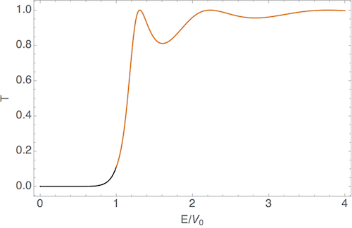
Here I show the two solutions for \( E/V_0 < 1 \) and \( E/V_0 > 1 \) joined together for some arbitrary numerical values; notice the transmission resonances at positive \( E/V_0 \).
Example 3: the square well
Another very interesting example is obtained by simply inverting the barrier, i.e. taking \( V_0 \) to \( -V_0 \); this gives us the square well potential:
\[ \begin{aligned} V(x) = \begin{cases} -V_0, & |x| < a \\ 0, & |x| > a. \end{cases} \end{aligned} \]
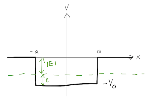
We'll begin with the case where \( -V_0 < E < 0 \). If we let \( \epsilon = E + V_0 = V_0 - |E| \) be the distance between the energy and the bottom of the well, then the wave number inside the well is the usual \( k = \sqrt{2m\epsilon} / \hbar \). The exponential decay constant outside the well is \( \kappa = \sqrt{2m|E|} / \hbar \).
States which satisfy this condition are known as bound states, since they propagate as plane waves inside the well but are exponentially damped outside. We can think of these states as being "bound" to the well, since their position is localized to the potential well (and slightly outside.)
The parity operator
In principle, we have four boundary conditions to match again. However, this is a good point to start letting symmetry make our lives easier. Notice that the potential well is symmetric under reversal around \( x=0 \), i.e. \( x \rightarrow -x \). This mirror reflection symmetry is more commonly known as parity. We can step back and more formally construct the parity operator as a unitary transformation which flips the sign of the position operator:
\[ \begin{aligned} \hat{P}{}^\dagger \hat{\vec{x}} \hat{P} = -\hat{\vec{x}}. \end{aligned} \]
(In fact, there's nothing special about the \( \hat{\vec{x}} \) operator and parity; we expect that mirror reflection should reverse the direction of any vector in space, so it will do the same to other spatial-vector operators.)
The parity operator has to be unitary: we can see that by applying it to the dot product of two vectors, which should itself be invariant under parity:
\[ \begin{aligned} \hat{P}{}^\dagger \hat{\vec{x}} \hat{P} \cdot \hat{P}{}^\dagger \hat{\vec{x}} \hat{P} = \hat{\vec{x}} \cdot \hat{\vec{x}} = \hat{P}{}^\dagger (\hat{\vec{x}} \cdot \hat{\vec{x}}) \hat{P} \end{aligned} \]
so \( \hat{P}^\dagger = \hat{P}^{-1} \). If the operator \( \hat{\vec{x}} \) transforms as above, then its eigenstates transform as well, \( \ket{\vec{x}} \rightarrow \hat{P}^\dagger \ket{\vec{x}} = \ket{-\vec{x}} \), and so
\[ \begin{aligned} \psi(\vec{x}) = \sprod{\vec{x}}{\psi} \rightarrow \bra{\vec{x}} \hat{P} \ket{\psi} = \sprod{-\vec{x}}{\psi} = \psi(-\vec{x}). \end{aligned} \]
In fact, from the states it's easy to see that \( \hat{P} \) is more than just unitary: if we apply parity twice, then
\[ \begin{aligned} \hat{P}{}^\dagger \hat{P}{}^\dagger \ket{\vec{x}} = \hat{P}{}^\dagger \ket{-\vec{x}} = \ket{+\vec{x}} \end{aligned} \]
so we also have \( \hat{P} = \hat{P}^{-1} \), i.e. \( \hat{P}^2 = \hat{1} \). (If you are familiar with group theory, this last property indicates that the symmetry group associated with parity is \( \mathbb{Z}_2 \). More on symmetry and groups later on.)
The action of parity on the Hamiltonian is particularly interesting. If we find that \( [\hat{P}, \hat{H}] = 0 \), then we will be able to construct simultaneous eigenkets of \( \hat{P} \) and \( \hat{H} \). Multiplying the commutator on the left by \( \hat{P}^\dagger \), we find that the commutator vanishing is equivalent to the condition
\[ \begin{aligned} \hat{H} = \hat{P}{}^\dagger \hat{H} \hat{P}, \end{aligned} \]
i.e. the Hamiltonian should be invariant under the action of parity. The momentum part of the Hamiltonian is proportional to \( \vec{p} \cdot \vec{p} \), and as we saw above, the dot product of a vector with itself is parity invariant, so \( \hat{H} \) is invariant if the potential is invariant, \( V(\vec{x}) = V(-\vec{x}) \).
For a potential satisfying this condition (like our square well), any eigenket of \( \hat{H} \) is also an eigenket of \( \hat{P} \). What do the parity eigenstates look like? If \( \ket{P} \) is a parity eigenstate, then we have
\[ \begin{aligned} \hat{P} \ket{P} = P \ket{P}. \end{aligned} \]
But
\[ \begin{aligned} \hat{P}{}^2 \ket{P} = P \hat{P} \ket{P} = P^2 \ket{P} = \ket{P} \end{aligned} \]
so \( P^2 = 1 \), i.e. \( P = \pm 1 \). Any energy eigenfunction \( \psi(x) \) can therefore be identified as either a positive-parity or even state, with \( P=1 \), or a negative-parity or odd state with \( P=-1 \). We can see what this implies for the spatial wavefunctions: if \( \ket{\psi} \) is an energy/parity eigenstate, then
\[ \begin{aligned} \sprod{x}{\psi} = \bra{x} \hat{P} \hat{P} \ket{\psi} = P \sprod{-x}{\psi}. \end{aligned} \]
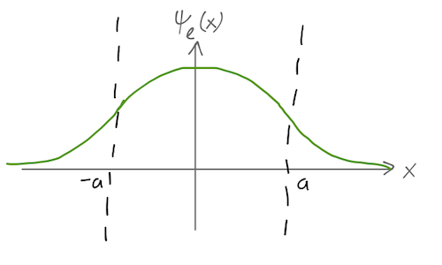
So in other words, the even-parity wavefunctions satisfy
\[ \begin{aligned} \psi_e(\vec{x}) = \psi_e(-\vec{x}) \end{aligned} \]
and the odd-parity ones satisfy
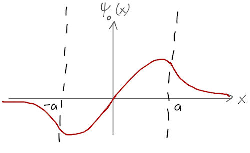
\[ \begin{aligned} \psi_o(\vec{x}) = - \psi_o(-\vec{x}). \end{aligned} \]
Back to our square well example. Because the potential is symmetric in \( x \), parity commutes with our Hamiltonian, and so we can split the solutions into those with even parity,
\[ \begin{aligned} \psi_e(x) = \begin{cases} A \cos kx, & |x| < a; \\ B e^{-\kappa |x|}, & |x| > a. \end{cases} \end{aligned} \]
and those with odd parity,
\[ \begin{aligned} \psi_o(x) = \begin{cases} A' \sin kx, & |x| < a; \\ B' e^{-\kappa x}, & x > a; \\ -B' e^{\kappa x}, & x < a. \end{cases} \end{aligned} \]
So we've immediately reduced our unknown coefficients from 4 down to 2. We've also reduced the number of constraints from continuity to 2, since continuity of \( \psi(x) \) and its derivative at \( x = +a \) now also guarantees it at the reflected boundary \( x = -a \). There is one more constraint, overall normalization of the wavefunction; only certain values of the energy \( E \) will allow us to satisfy all constraints.
Next time: we find those bound states, and back to the S-matrix.