At the end of last time, we were finishing up our solution for bound states in the square well. We had just appealed to parity symmetry to separate the energy eigenfunction solutions into even and odd parity. Recall that the most general even-parity solution takes the form
\[ \begin{aligned} \psi_e(x) = \begin{cases} A \cos kx, & |x| < a; \\ B e^{-\kappa |x|}, & |x| > a. \end{cases} \end{aligned} \]
Applying the boundary condition at \( x=a \) (the other boundary is redundant) to this state gives
\[ \begin{aligned} A \cos ka = B e^{-\kappa a} \\ -Ak \sin ka = -B\kappa e^{-\kappa a} \end{aligned} \]
which can be combined to obtain a condition on the wave numbers and thus the allowed energy \( E \):
\[ \begin{aligned} ka \tan ka = \kappa a. \end{aligned} \]
Similarly, for the odd-parity states we find
\[ \begin{aligned} ka \cot ka = -\kappa a. \end{aligned} \]
Now let's define for convenience the parameters \( \xi \equiv ka \) and \( \eta \equiv \kappa a \). From the definitions of \( k \) and \( \kappa \), we see that
\[ \begin{aligned} \xi^2 + \eta^2 = \frac{2ma^2}{\hbar^2} (E + V_0 - E) = \frac{2ma^2}{\hbar^2} V_0, \end{aligned} \]
while from above we have (for even parity)
\[ \begin{aligned} \xi \tan \xi = \eta. \end{aligned} \]
This is a transcendental equation, so we can't find a closed-form solution. However, we can solve this pair of equations graphically. If we plot \( \eta \) vs. \( \xi \), then the first equation above defined a circle with radius \( \sqrt{2mV_0} a/\hbar \); solutions occur wherever this circle intersects the function \( \xi \tan \xi \).
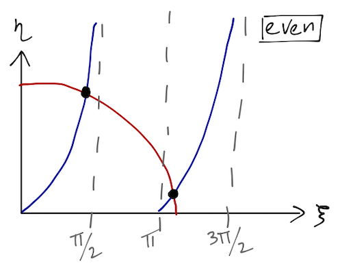
These are solutions for the bound-state energy \( E \), which determines the values of \( k \) and \( \kappa \). Notice that even as the radius of the circle vanishes, we will always find at least one even-parity bound state. As the radius rises (the well becomes deeper or wider), the number of solutions increases. If we take \( V_0 \rightarrow \infty \) then we find an infinite number of bound-state solutions, corresponding to the (even-parity) standard results for the infinite square well.
What about the odd-parity solutions? We have the same equation for the circular curves, but now the boundary conditions instead yield the relation
\[ \begin{aligned} \xi \cot \xi = -\eta. \end{aligned} \]
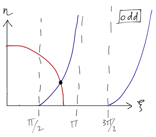
Now we see that there will be no solutions if \( \sqrt{2mV_0} a/\hbar < \pi/2 \); if the potential well is too shallow, there are no odd-parity bound states.
For completeness, I'll note that we can also study scattering from the square well, i.e. solutions with \( E>0 \). We will find similar results to what we had for the barrier before: I won't go through the details, but in particular we find for the transmission coefficient
\[ \begin{aligned} T = \left(1 + \frac{\sin^2(2k'a)}{4E/V_0(E/V_0+1)} \right)^{-1}. \end{aligned} \]
so we once again have resonance at precisely the values \( 2k'a = n\pi \). (However, note that the definition of \( k' \) has changed: for the potential barrier we had \( k' = \sqrt{2m(E-V_0)}/\hbar \), while for the well it is \( k' = \sqrt{2m(E+V_0)}/\hbar \).)
We can think about this more physically to understand the source of the resonant behavior. Remember that at any barrier, a quantum-mechanical particle will undergo both transmission and reflection (this is possible because the wavefunction allows a single particle to be non-localized in a sensible way.) Although we've focused on the final transmission amplitude, there is generically transmission and reflection at both edges of the barrier. In particular, some part of the incident plane wave \( A \) will be reflected internally some number of times before finally being transmitted into outgoing wave \( F \). The condition \( 2k'a = n\pi \) can be rewritten as
\[ \begin{aligned} 4a = n (2\pi/k'), \end{aligned} \]
in other words, transmission resonance occurs when the distance \( 4a \) traveled by an internally reflected wave is equal to an integer multiple of the de Broglie wavelength \( (2\pi/k') \), resulting in constructive interference.
Bound states and zero-point energy
What we have found is that a quantum mechanical potential with bound states has only a discrete set of solutions, corresponding to particular values of the energy \( E \) (the energy is quantized.) Quantization of energy is a very important quantum phenomenon, and in fact is more general than just our square-well example. If we suppose we have some arbitrary potential well which is negative in some range, with \( V=0 \) away from the well, then the solutions for bound states \( E<0 \) must take the form (for large, positive \( x \))
\[ \begin{aligned} \psi(x) = B e^{\kappa x} + C e^{-\kappa x} \end{aligned} \]
The coefficients \( B \) and \( C \) are determined by continuity of the wavefunction and its derivative at the boundary of the well. But for \( x \rightarrow +\infty \), the first term is not normalizable, so the only possible wavefunctions are those which satisfy the equation
\[ \begin{aligned} B(E) = 0. \end{aligned} \]
This is the source of quantization; the function \( B(E) \) is itself continuous, but will generally only have a finite number of zeroes. This is similar to how quantization arises in classical physics - wave modes must satisfy some boundary condition, e.g. for electromagnetic waves in a cavity or a string tied between two posts. But in quantum mechanics, everything is a wave, so the effect occurs more often.
If you go on to find particular solutions for some specific numerical values here, or if you think back to the energy bound states for the infinite square well or the harmonic oscillator, you will recall that in each of those examples the ground-state (lowest) energy eigenvalue \( E_0 \) was somewhat larger than the minimum of the potential. This is, in fact, a very general effect of quantum mechanics: the ground-state energy is strictly greater than the minimum of the potential. In other words, there is always some "zero-point energy".
We can see why this should be true in general. In an energy eigenstate, we can divide the energy up into the expectation values of kinetic and potential energy:
\[ \begin{aligned} E = \ev{\hat{T}} + \ev{\hat{V}}. \end{aligned} \]
In terms of the energy eigenstate wavefunction, we can write
\[ \begin{aligned} \ev{\hat{T}} = \ev{\frac{\hat{p}^2}{2m}} = - \frac{\hbar^2}{2m} \int_{-\infty}^\infty dx\ \psi^\star(x) \frac{d^2}{dx^2} \psi(x) \\ = \frac{\hbar^2}{2m} \int_{-\infty}^\infty dx \left| \frac{d\psi}{dx} \right|^2 \end{aligned} \]
where we have integrated by parts to move one of the derivatives onto \( \psi^\star(x) \), and discarded the "boundary term" using the requirement that \( \psi(x) \) goes to zero as \( x \rightarrow \infty \). The mean potential energy is easier to find:
\[ \begin{aligned} \ev{\hat{V}} = \int_{-\infty}^\infty dx\ V(x) |\psi(x)|^2. \end{aligned} \]
The kinetic energy is the integral of a squared absolute value, so \( \ev{\hat{T}} > 0 \) always (the only possible exception is \( d\psi/dx = 0 \), which would imply the wavefunction is just zero everywhere.) On the other hand,
\[ \begin{aligned} \ev{V} = \int_{-\infty}^\infty V(x) |\psi(x)|^2 \geq \int_{-\infty}^\infty V_{\rm min} |\psi(x)|^2 = V_{\rm min}. \end{aligned} \]
where \( V_{\rm min} \) is the global minimum value of \( V(x) \). So \( E = \ev{T} + \ev{V} > V_{\rm min} \). The observation that bound states in a potential well correspond to \( -V_0 < E < 0 \) isn't too surprising; after all, the same statement is almost true classically. The difference is in the left inequality, that \( E \) is strictly greater than the potential minimum. A classical particle can have \( E = -V_0 \), corresponding to being at rest at position \( x_0 \) where \( V(x) \) is minimized. A quantum particle, on the other hand, cannot have \( E = -V_0 \); as you might suspect, the reason has to do with the uncertainty principle.
What does the state of minimum potential energy look like, quantum mechanically? Since (from above) \( \ev{V} \) is just a weighted average of \( V(x) \) with the probability density given by the squared wavefunction, minimizing \( V(x) \) means localizing the wavefunction about the minimum. In fact, we will only have \( \ev{V} = -V_0 \) when the wavefunction is squeezed into a delta function, \( |\psi(x)|^2 = \delta(x) \).
This localized wavefunction will have \( \Delta x \) very small, which means that by the uncertainty principle the spread in momentum \( \Delta p \) is very large. But this means that
\[ \begin{aligned} \ev{\hat{p}{}^2} = (\Delta p)^2 + \ev{\hat{p}}{}^2 \geq (\Delta p)^2. \end{aligned} \]
So the harder we try to minimize the potential \( \ev{V} \), the larger the average kinetic energy \( \ev{T} = \ev{\hat{p}^2} / 2m \) becomes! The uncertainty relation between \( \Delta x \) and \( \Delta p \) ensures that a quantum particle can never be at rest at the bottom of a potential well, so there will always be some zero-point energy.
Scattering theory
Let's return to a more general discussion of scattering theory and the \( S \)-matrix, and then we'll come back and finish with scattering from the square well. The general discussion will help us appreciate some features that would otherwise look very mysterious! For this part I'm going to be following some excellent lecture notes by Prof. David Tong which go through scattering theory in a lot more detail. (As David points out for motivation, this isn't just a discussion relevant for particle physics: scattering experiments are everywhere in physics. You looking at the blackboard right now is a scattering experiment!)
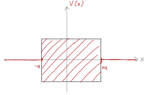
We can start by thinking about a very general case where we have a "black box" target potential near the origin; let's say it's an arbitrary function but still restricted to exist in the range \( |x| < a \). We thus know that outside the black box region, we still have simple plane-wave solutions:
\[ \begin{aligned} \psi(x) = \begin{cases} A e^{ikx} + Be^{-ikx}, & (x < -a); \\ {\rm (something\ messy)}, & (-a < x < a); \\ F e^{ikx} + Ge^{-ikx}, & (x > a). \end{cases} \end{aligned} \]
This is a little simplified, since we're assuming a sharp cutoff on the black box region. If you like, you can think of the two plane-wave solutions as being asymptotic behavior for \( x \rightarrow \pm \infty \).
We can still define the S-matrix that related the incoming coefficients \( A \) and \( G \) to the outgoing ones \( B \) and \( F \):
\[ \begin{aligned} \left( \begin{array}{c} F \\ B \end{array} \right) = \left( \begin{array}{cc} S_{11} & S_{12} \\ S_{21} & S_{22} \end{array} \right) \left( \begin{array}{c} A \\ G \end{array} \right). \end{aligned} \]
(Note that the way David Tong chooses to define his S-matrix is ever so slightly different, but nothing substantial changes in my version.) Let's be a little more concrete about what the entries in S really are. For example, the upper row gives the relation
\[ \begin{aligned} F = S_{11} A + S_{12} G. \end{aligned} \]
Remember that if we introduce time dependence, \( A \) and \( G \) represent incoming particles from the left and the right respectively. We think of these coefficients are being inputs under our experimental control. If we have \( G=0 \), then \( S_{11} = F/A \equiv t \) is the ratio of transmitted to incoming amplitude - i.e. we would have for the transmission coefficient \( T = |t|^2 \). On the other hand, if we switch off \( A \) then \( S_{12} = F/G \equiv r' \) gives the reflected wave amplitude, and reflection coefficient \( R' = |r'|^2 \). (I'm using primes to distinguish the G experiment from the A experiment.)
Using this language, we can rewrite the S-matrix as
\[ \begin{aligned} {S} = \left( \begin{array}{cc} t & r' \\ r & t' \end{array} \right). \end{aligned} \]
Remembering that this should be unitary, we should check the expression
\[ \begin{aligned} {S}^\dagger {S} = \left( \begin{array}{cc} |t|^2 + |r|^2 & tr'^\star + rt'^\star \\ t^\star r' + r^\star t' & |t'|^2 + |r'|^2 \end{array} \right) \end{aligned} \]
The two diagonal entries are equal to \( T + R \) and \( T' + R' \), and so are both 1 by conservation of probability. It's not so obvious that the off-diagonal entries vanish, but as long as \( V(x) \) is a real function it's possible to prove (see the linked notes) that
\[ \begin{aligned} t' = t,\ r' = -\frac{r^\star t}{t^\star} \end{aligned} \]
which relates the two scattering experiments and ensures that S is indeed unitary.
Now, there are some nice features to working in the parity basis in general: we could redefine our asymptotic scattering states in terms of parity-even and parity-odd combinations. In particular, in the parity basis the S-matrix is diagonal for potentials \( V(x) \) that are symmetric about \( x=0 \), and in such a situation it can be shown that the scattering is entirely captured by phase shifts of the outgoing waves relative to the incoming ones. That discussion is useful but slightly technical, so I'll leave it for you to read on your own, and instead we'll dive into what David calls "the magic of the S-matrix".
The S-matrix and bound states
First of all, note that the S-matrix is a function of the momentum \( k \) of our asymptotic scattering states: we should write it as \( {S}(k) \) and its entries as \( t(k) \) and \( r(k) \). (There's only one momentum \( k \), because whatever happens inside the black box we assume that it's energy conserving.) As long as \( E > 0 \) we know that \( k \) will be real; as \( k \rightarrow \infty \), we expect that \( {S}(k) \) goes to the identity matrix, since for a sufficiently energetic particle the potential will have little effect and we expect the transmission coefficient \( T \rightarrow 1 \).
What about the case where \( E < 0 \)? At first glance this would seem to have nothing to do with the S-matrix, because the plane-wave form of our solutions to the Schrödinger equation becomes invalid at asymptotic \( x \). However, that's not entirely true: from a mathematical point of view, the Schrödinger equation in regions where \( V=0 \) simply looks like
\[ \begin{aligned} \psi''(x) = -\frac{2mE}{\hbar^2} \psi(x) = -k^2 \psi(x) \end{aligned} \]
where the latter definition is still perfectly fine if \( E < 0 \), as long as we allow \( k \) to be imaginary. If \( k \equiv i\kappa \) where \( \kappa \) is real, then we have for our asymptotic solutions
\[ \begin{aligned} \psi(x) = \begin{cases} Ae^{-\kappa x} + (rA+t'G) e^{\kappa x}, & (x \rightarrow -\infty); \\ (tA+r'G) e^{-\kappa x} + Ge^{\kappa x}, & (x \rightarrow +\infty). \end{cases} \end{aligned} \]
We see a problem right away: two of the exponential solutions blow up at infinite \( x \) and are not normalizable! The appropriate limit to remove the divergent parts of our solutions is \( A, G \rightarrow 0 \). But then since \( A \) and \( G \) appear in every term in the solution, we either have no solution (\( \psi(x) = 0 \)), or the S-matrix entries must diverge at the same time as \( A \) and \( G \) vanish, so that the combinations in front of the well-behaved exponential terms are finite.
In other words, thinking of \( {S}(k) \) as a function of the complex wave number \( k \), the behavior of \( {S}(k) \) along the real axis tells us about asymptotic scattering states with positive energy, but we can get even more: bound states can be identified as poles of \( {S}(k) \) along the imaginary axis.
(You might complain that talking about poles of a matrix is imprecise; if you like, the correspondence is with poles in the eigenvalues of \( {S}(k) \). The discussion is cleaner in the parity eigenbasis, where \( {S} \) becomes diagonal for symmetric potentials and the poles are cleanly related to parity-even and parity-odd bound states.)
The fact that both the real and imaginary parts of \( S(k) \) contain interesting physics information about a given potential should make us wonder whether there is anything else interesting hidden in the complete structure of \( S(k) \) continued into the complex plane. In fact, there is: the phenomenon of resonance can be understood in terms of poles structure at complex \( k \).
It's easiest to understand this part of the discussion if we work backwards. Assume that \( S(k) \) has a pole at the complex value \( k_0 - i \gamma \), where \( \gamma > 0 \) (this will turn out to be the interesting case.) We can work backwards to obtain the energy of the state from \( k \):
\[ \begin{aligned} E = \frac{\hbar^2 k^2}{2m} = \frac{\hbar^2 (k_0^2 - \gamma^2)}{2m} - 2i \frac{\hbar^2 \gamma k_0}{2m} \equiv E_0 - \frac{i\Gamma}{2}. \end{aligned} \]
So the energy is complex. Your first reaction might be "obviously this is unrealistic" - either because you know on physical grounds that energy should be real, or because we've said the Hamiltonian is Hermitian and so its eigenvalues should be real. But let's ignore that for the moment and ask what a complex energy might mean. The simplest way to understand what's happening is to consider the time-dependence of such a state: we will have
\[ \begin{aligned} \psi(x,t) \sim e^{-iEt/\hbar} \psi(x) = e^{-iE_0 t/\hbar} e^{-\Gamma t/2\hbar} \psi(x). \end{aligned} \]
In addition to the usual phase, we have exponential decay of the entire state! We would similarly find that the probability density is decaying exponentially (you'll look at this on the homework a bit.) To think about asymptotic behavior in this case, it's helpful to restore the spatial dependence: for example, for the transmitted part of the solution as \( x \rightarrow \infty \), we have
\[ \begin{aligned} \psi(x,t) \sim e^{ikx} e^{-iEt/\hbar} = e^{ik_0 x} e^{-iE_0 t/\hbar} \exp \left[ \gamma x - \frac{\Gamma t}{2\hbar}\right] \\ = (...) \exp \left[ \gamma (x - vt) \right], \end{aligned} \]
where
\[ \begin{aligned} v = \frac{\Gamma}{2\hbar \gamma} = \frac{\hbar k_0}{m} \end{aligned} \]
is the linear speed determined by the (real) energy and mass of our particle. Ignoring details of how to construct a particular solution, the interpretation is clear: the asymptotic solution behaves like a free particle, translating to the right at speed \( v \)! (We'll find a similar solution on the left.)
We've now seen enough math to assign a physical interpretation. As we discussed above, poles in \( S(k) \) indicate the energy values that correspond to bound states. These are generally on the imaginary-\( k \) axis, corresponding to \( E<0 \), since the solution must not exist asymptotically for the particle to be truly bound. But we could easily imagine a potential which consists of a large and deep well, but not an infinitely deep one:
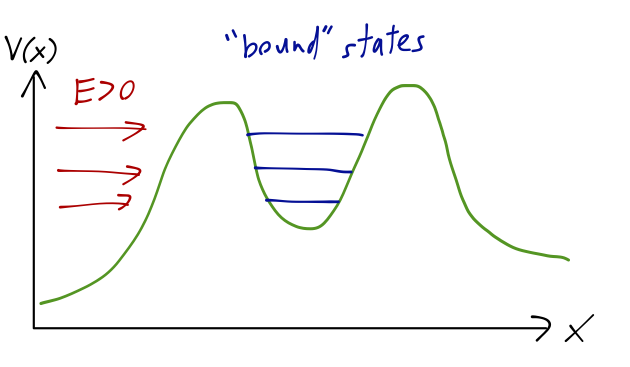
We might expect to find "bound states" here if the well is deep and wide enough and we ignore the outside. But the presence of the lower-energy region outside the well means any such states must be unstable! If we imagine an initial state with our particle trapped inside the well, it will have some finite probability per unit time to tunnel through the barrier and escape; if we wait long enough, it will definitely escape. This is exactly the situation described by a complex energy eigenvalue above: the local wavefunction \( \psi(x,t) \) within the well decays exponentially to zero, and the wavefront outside the well moves away with some linear speed.
(Note that this explanation requires \( \gamma > 0 \), i.e. the poles to be in the lower half-plane; otherwise we would have exponential growth instead of decay, which would not match on to this experimental situation anymore.)