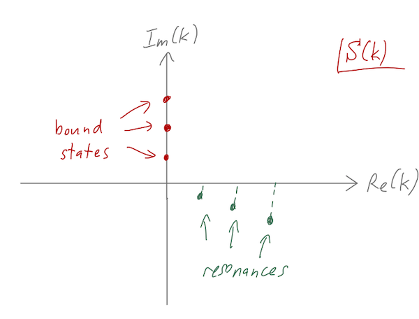
Last time, we were digging in to the complex structure of the S-matrix. We discovered first that poles on the imaginary \( k \)-axis (corresponding to negative energy) determine the locations of bound states. Then we moved on to consider complex \( k \) in full generality, finding that \( k = k_0 - i \gamma \) implies time dependence that decays exponentially, and asymptotically resembles a free particle:
\[ \begin{aligned} \psi(x,t) \sim e^{-iE_0 t/\hbar} e^{-\Gamma t/(2\hbar)} \psi(x) \rightarrow (...) \exp \left[ \gamma (x - (\hbar k_0/m) t) \right]. \end{aligned} \]
This matches up nicely with the interpretation of unstable "bound" states inside a large potential well:
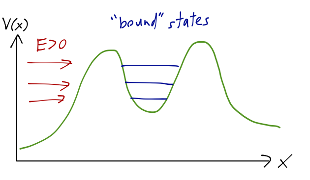
The energy levels inside the well are also known as resonances. They can indeed be identified as complex poles in the \( S \)-matrix. Of course, if we probe the well by carrying out a scattering experiment and measuring the transmission coefficient \( T \), we will only be studying \( S(k) \) on the positive real axis, so we will never see a divergence in \( T \). However, it's easy to see that the presence of nearby complex poles will cause local maxima in \( T \) - precisely the phenomenon of transmission resonance that we noted before.
We can go a step further and see precisely how a pole would cause a transmission resonance. Let's think in terms of energy instead of \( k \) this time: suppose the transmission amplitude \( t(E) \) has a pole at \( E = E_0 - i\Gamma/2 \) as above. Close enough to the pole, it will dominate over all other contributions:
\[ \begin{aligned} t(E) \approx \frac{Z}{E - E_0 - i\Gamma/2}, \end{aligned} \]
where \( Z \) is the residue of the pole. The transmission coefficient for real \( E \) is then equal to
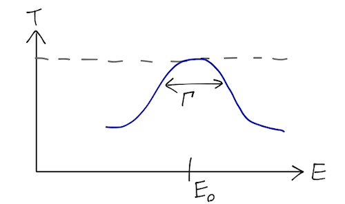
\[ \begin{aligned} T(E) \approx \frac{|Z|^2}{(E-E_0)^2 + \Gamma^2/4}. \end{aligned} \]
This should look familiar: this is exactly the same Lorentzian distribution that we saw in magnetic resonance. The peak is at \( E_0 \), and the parameter \( \Gamma \) is known as the width of the Lorentzian, because it corresponds to the width of the peak (strictly, the "full-width at half-max", i.e. the distance between the points halfway down from the peak):
The Lorentzian isn't always a great approximation, depending on how far away the closest pole is and how many other poles are nearby, but it always works if we're "close enough" to a single pole.
I'll emphasize once again that actually interpreting complex energies as "physical" states is a phenomenological concept. Strictly speaking, in quantum mechanics probability is conserved, Hamiltonians are Hermitian, and there are no complex energy eigenvalues. But if we look at a local part of a whole system, like the inside of a potential well, then we can approximate the behavior by making use of complex energies. Probability conservation is lost, but just because we've restricted our attention - we know the lost probability flows out of the well and into asymptotic states.
The potential step and the S-matrix
Now, some painful algebra! Let's do a unified treatment of the well and the barrier that I'll call the potential step, where we have constant \( V_0 \) for \( |x| < a \) but the sign of \( V_0 \) is left arbitrary. We can write the general solution as
\[ \begin{aligned} \psi(x) = \begin{cases} A e^{ikx} + Be^{-ikx}, & (x < -a); \\ C e^{ik'x} + De^{-ik'x}, & (-a < x < a); \\ F e^{ikx} + Ge^{-ikx}, & (x > a). \end{cases} \end{aligned} \]
where \( k = \sqrt{2mE} / \hbar \) and \( k' = \sqrt{2m(E-V_0)} / \hbar \) will be complex in general. They are, of course, not independent - we recognize immediately that
\[ \begin{aligned} k'^2 = \frac{2m(E-V_0)}{\hbar^2} = k^2 - \frac{2mV_0}{\hbar^2}. \end{aligned} \]
At the left boundary, we have the equations
\[ \begin{aligned} A e^{-ika} + Be^{ika} = Ce^{-ik'a} + De^{ik'a} \\ kA e^{-ika} - kBe^{ika} = k'C e^{-ik'a} - k'D e^{ik'a} \end{aligned} \]
and at the right boundary,
\[ \begin{aligned} C e^{ik'a} + De^{-ik'a} = Fe^{ika} + Ge^{-ika} \\ k'C e^{ik'a} - k'D e^{-ik'a} = kFe^{ika} - kGe^{-ika} \end{aligned} \]
Letting Mathematica do the algebra for us, we find the results
\[ \begin{aligned} t = \frac{4kk' e^{-2i(k-k')a}}{e^{4ik'a} (k-k')^2 - (k+k')^2} \\ r = \frac{2i (k-k')(k+k') \sin(2k'a) e^{-2i(k-k')a}}{e^{4ik'a} (k-k')^2 - (k+k')^2} \end{aligned} \]
Let's check against what we had previously: for the potential step with \( V_0 > 0 \) and scattering with \( 0 < E < V_0 \), we have \( k' = i\kappa \) for real \( \kappa \) and find the transmission coefficient
\[ \begin{aligned} T = \frac{8k^2 \kappa^2}{(k^2 + \kappa^2)^2 \cosh (4\kappa a) - (k^4 - 6k^2 \kappa^2 + \kappa^4)} \end{aligned} \]
which, although not obviously, exactly matches on to the expression we found before.
Now we can talk about structure in the complex plane! We see that both \( t \) and \( r \) have poles for any \( k \) satisfying the equation
\[ \begin{aligned} e^{4ik'a} (k-k')^2 - (k+k')^2 = 0, \end{aligned} \]
yielding two solutions,
\[ \begin{aligned} k = k' \frac{e^{2iak'}-1}{e^{2iak'}+1},\ \ k= k' \frac{e^{2iak'}+1}{e^{2iak'}-1}. \end{aligned} \]
Now let's narrow things down. Suppose first that \( k' \) is real, which means that \( E-V_0 > 0 \). Then we can simplify using trig identities to the relations
\[ \begin{aligned} k = ik' \tan k'a,\ \ k = -ik' \cot k'a. \end{aligned} \]
These right-hand sides are pure imaginary; if \( E > 0 \), then \( k \) is real and there are no poles in the transmission coefficient (good news!) On the other hand, if \( E < 0 \) we have poles that we know should correspond to bound states, and indeed we recover exactly the bound-state energy equations that we found above, e.g. \( \eta = \xi \tan \xi \)!
What about the other possibility, that \( k' \) is pure imaginary? (This corresponds to the case \( E < V_0 \).) If we identify \( k' = i \kappa \), then instead we find the two equations
\[ \begin{aligned} k = -\kappa \tanh \kappa a,\ \ k = -\kappa \coth \kappa a. \end{aligned} \]
In the \( k \) plane, these solutions must lie somewhere on the negative real axis; but since \( k \) is the square root of the (real) energy, it's either real and positive or imaginary and positive. (Letting \( k \) be negative will amount to flipping which solutions we think of as incoming and outgoing, which invalidates some assumptions we've made.) So there are no poles in the case of the potential barrier, which is good because a pole in the transmission coefficient with visible asymptotic states at \( x = \pm \infty \) would violate probability conservation badly!
We know that we can actually generalize completely to allow \( k \) to be in the complex plane. Finding the complex pole locations is not easy, so I will resort to a numerical treatment: we can plot \( t(k) \) in the complex plane for some simple numerical values \( a = 1 \), \( m = 1 \), and \( V_0 = \pm 1 \). Here's what we see:
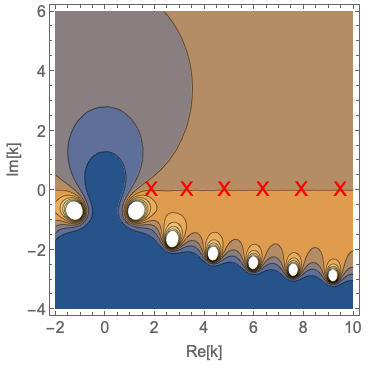
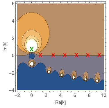
I've put the locations of the transmission resonances for positive/negative \( V_0 \) on the real axis (red X's), and the first bound-state energy solution for negative potential on the imaginary axis in the right plot (green X). We see that everyhting lines up pretty well! (The transmission resonances are not perfectly above the poles, but since the poles are relatively close together we wouldn't expect them to be; imagine adding together a sequence of increasingly broad Lorentzian curves.)
Example 4: The ammonia maser
Let's turn to a much more concrete example than these abstract square potentials: the ammonia molecule, \( NH_3 \). (We're still going to reduce it to a nice square potential, but at least the starting point is more concrete.)
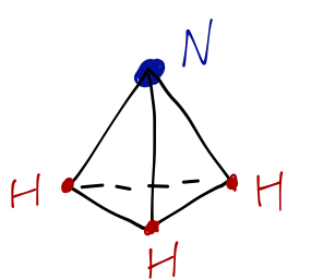
The structure of ammonia makes it a particularly interesting case, which is actually simpler than it looks. It is a rather complex molecule, a bound state consisting of a large number of protons, neutrons, and electrons arranged in a complicated way. But part of being a good physicist is knowing what the interesting behavior of a system is an isolating it.
What are the different possible states of an ammonia molecule? There are many possible ways for it to be put into an excited energy state: it can be moving through space at some speed, or rotating, or the molecular bonds could be vibrating. The electrons, or even the neutrons and protons inside the nuclei, could also be in a higher energy state. Experimentally, we're able to measure differences between these excited states and the ground state as emission lines, photons which carry away the energy difference.
What spectral lines do we see from ammonia? The shortest-range excitations correspond to the highest energy; exciting the individual electrons requires electron-volts (eV) of energy, corresponding to visible or ultraviolet photons (and nuclear excitations would give gamma rays.) Vibration of the molecular bonds has a lower energy, giving infrared photons; rotation of the entire molecule gives far-infrared.
There's one more possible excitation which we haven't considered, arising from the motion of the nitrogen relative to the hydrogen atoms. The pyramid shape of ammonia is fairly rigid, and is a local minimum of the overall potential energy among the four atoms. However, keeping the plane of the three \( H \) fixed, it's obvious that the \( N \) can be either above or below the plane with the same energy.
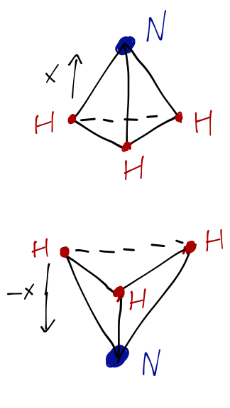
The motion in which the nitrogen switches from above to below the hydrogen plane is known as inversion. Inversion has the lowest energy of all, giving rise to microwave photons. Microwave lines are interesting because they are relatively unusual, and the ammonia line is very important in radio astronomy.
This isn't really a vibrational mode in the normal sense; vibration comes from small deformations around an equilibrium point, but here there is quite a large potential barrier between the two inverted configurations. If we take the \( N \) atom to be fixed (since it's heavy) and let \( x \) be the distance from the \( N \) to the plane of the hydrogen atoms, then the potential energy \( V(x) \) looks something like this:
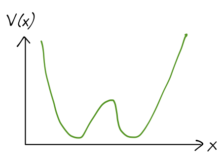
So studying inversion is a one-dimensional problem (now involving the mass of a fictitious particle, the reduced mass \( 3m_H m_N / (3m_H + m_N) \).) In fact, we'll further simplify our model by approximating the true potential with a rectangular one:
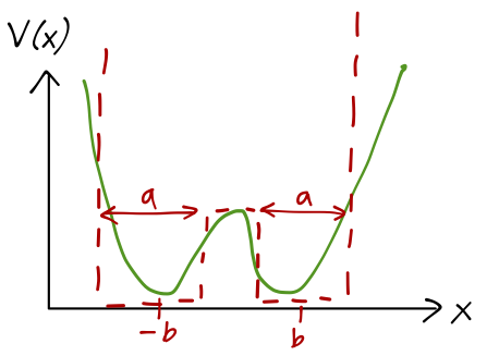
\[ \begin{aligned} V(x) = \begin{cases} V_0, & |x| \leq b-a/2; \\ 0, & b-a/2 < |x| < b+a/2; \\ \infty, & |x| \geq b+a/2. \end{cases} \end{aligned} \]
This will be good enough to gain a qualitative understanding of the physics. The ground state energy will be some \( E \) such that \( 0 < E < V_0 \); inversion corresponds to tunneling of the system through the potential barrier.
Infinite potential barrier
To really understand the tunneling effect, it's useful to start by taking \( V_0 \rightarrow \infty \) as well, so that tunneling is impossible. Then the problem reduces to a double infinite square-well potential. I'll remind you that the energy eigenvalues for a particle of mass \( m \) in an infinite square well of width \( a \) are
\[ \begin{aligned} E_n = \frac{\hbar^2 k_n^2}{2m} \end{aligned} \]
where \( k_n = n\pi/a \). The boundary conditions are simple: the wavefunction is zero inside the infinite barriers, and so it must vanish at the borders. We can write two possible wavefunctions that aren't zero everywhere:
\[ \begin{aligned} \psi_L^n(x) = \begin{cases} \sqrt{\frac{2}{a}} \sin \left[ k_n \left(b + a/2 + x\right) \right], & b-a/2 < -x < b+a/2 \\ 0, & {\rm elsewhere}; \end{cases} \\ \psi_R^n(x) = \begin{cases} \sqrt{\frac{2}{a}} \sin \left[ k_n \left(b + a/2 - x\right) \right], & b-a/2 < x < b+a/2 \\ 0, & {\rm elsewhere}; \end{cases} \end{aligned} \]
These are just the wavefunctions for the particle being either in the left box or the right box; there is a two-fold degeneracy in the energy eigenvalues, since \( \psi_1^n(x) \) and \( \psi_2^n(x) \) have the same energy if \( n \) is the same.
Even with the infinite potential barrier, there are excited states, and we should expect to find a spectral line for e.g. the \( n=2 \) to \( n=1 \) transition with frequency \( (E_2 - E_1) / \hbar \). This isn't what we're looking for, and in fact is simply a vibrational mode in which the three \( H \) atoms move together in small displacement around their equilibrium. Like the other vibrational modes, this gives an infrared emission line.
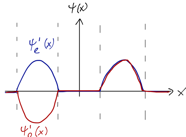
We can take our localized wavefunctions and recombine them with parity in mind as even and odd wavefunctions
\[ \begin{aligned} \psi_e^n(x) = \frac{1}{\sqrt{2}} [\psi_L^n(x) + \psi_R^n(x)] \\ \psi_o^n(x) = -\frac{1}{\sqrt{2}} [\psi_L^n(x) - \psi_R^n(x)] \end{aligned} \]
You can think of this as a sort of "change of basis": it's clear that any wavefunction can be expressed either in terms of the individual well eigenstates, or these parity-eigenfunction combinations.
Next time: we lower the middle barrier and solve the system.