Last time, we were discussing the emission spectrum of the ammonia molecule, specifically inversion which is a kind of motion in which the nitrogen atom swaps places:
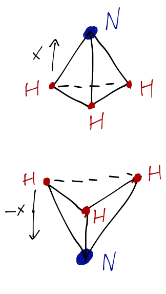
We argued that the potential as a function of \( x \), the distance from the nitrogen to the plane of the \( H_3 \), can be modeled approximately as a double square well:
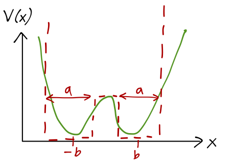
For the limit that the central barrier height \( V_0 \rightarrow \infty \), we just have a pair of infinite square wells that don't interact at all. We noted that we can divide their solutions into even-parity and odd-parity wavefunctions, which are a simple linear combination of the wavefunctions within the two wells.
Finite potential barrier
(I'll go fast through parts of this. If you don't see how I arrived at a particular equation, I encourage you to derive them yourself; start with the most general combination of plane waves and exponentials, and apply the boundary conditions and parity!)
Now we lower the center potential barrier to some finite value \( V_0 \), assuming we have \( E < V_0 \). The outer barriers are still infinite, so the wavefunction still has to vanish there, which means it takes the general form in the two wells
\[ \begin{aligned} \psi(x) = \begin{cases} A \sin \left[ k (b + a/2 - x) \right],& b-a/2 < x < b+a/2; \\ A' \sin \left[ k (b + a/2 + x) \right],& b-a/2 < -x < b+a/2. \end{cases} \end{aligned} \]
Since parity is still a good symmetry of the potential, all possible solutions will divide into the even-parity set \( A_e = A'_e \), and the odd-parity set \( A_o = -A'_o \). There will be a corresponding set of bound-state energies \( E_e \) and \( E_o \), with corresponding wave numbers \( k_e, k_o \).
There is now also a non-zero wavefunction inside the central barrier. If we define the usual \( \kappa = \sqrt{2m(V_0-E)} / \hbar \), then the even and odd wavefunctions inside the barrier are just symmetric and anti-symmetric combinations of exponentials:
\[ \begin{aligned} \psi_e(x) = B_e \cosh (\kappa_e x), \\ \psi_o(x) = B_o \sinh (\kappa_o x). \end{aligned} \]
As always, we proceed by matching boundary conditions at \( x = \pm (b-a/2) \). For the even eigenfunctions, we find the pair of equations
\[ \begin{aligned} A_e \sin (k_e a) = B_e \cosh \left[ \kappa_e \left(b-a/2\right) \right] \\ -k_e A_e \cos (k_e a) = B_e \kappa_e \sinh [\kappa_e (b-a/2)] \end{aligned} \]
which we can divide one by the other to obtain
\[ \begin{aligned} \tan (k_e a) = -\frac{k_e}{\kappa_e} \coth [\kappa_e (b-a/2)]. \end{aligned} \]
The same exercise for the odd solutions gives the equation
\[ \begin{aligned} \tan (k_o a) = -\frac{k_o}{\kappa_o} \tanh [\kappa_o (b-a/2)]. \end{aligned} \]
Like the single potential well, we find that the wave numbers of the energy bound states satisfy transcendental equations, one for each parity eigenvalue. Unlike the single well, these equations are more complicated, since we now have transcendental functions on both sides. Given the appropriate experimental information on ammonia, we can always solve these equations numerically.
The key point, however, is that the equations are different, which means that where before we had two states with identical energy \( E_n \) (particle in the left well or right well), now the states have been split, with energies \( E_{e,n}, E_{o,n} \). We have broken a degeneracy by allowing tunneling between the wells. We can sketch a numerical solution for the lowest four energy states:
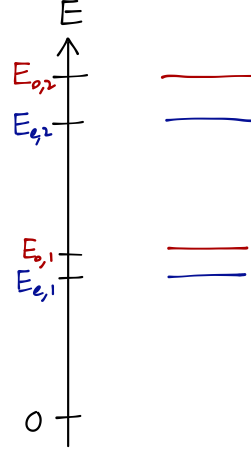
The parity splitting \( E_{o,1} - E_{e,1} \) is much smaller than the level splitting \( E_{e,2} - E_{e,1} \) (experimentally, by a factor of a thousand or so.) This smallest splitting corresponds exactly to inversion; to see precisely how, we need to go further and look at the time evolution of this system.
Bonus note: the zero-barrier limit
A question that came up during lecture: what happens to the system when \( V_0 \) becomes very small (or equivalently, what do the bound states look like for \( E \gg V_0 \)?) This limit isn't relevant for the study of ammonia inversion, but it's always a good idea to check your limits in any physics calculation.
In the limit that \( V_0 \) vanishes we expect to recover results for a single infinite square well of width \( 2b+a \). In fact, as soon as \( E > V_0 \) we have to be careful, since the solutions in the barrier region become plane waves, so we have to replace \( \kappa \rightarrow -ik' \), where \( k' = \sqrt{2m(E-V_0)}/\hbar \).
With this replacement, and the identities \( \coth(ix) = -i \cot(x) \) and \( \tanh(ix) = i \tan (x) \), we find the energy conditions become
\[ \begin{aligned} \tan (k_e a) = -\frac{k_e}{k'_e} \cot[-k'_e (b-a/2)] \\ \tan (k_o a) = +\frac{k_o}{k'_o} \tan[-k'_o (b-a/2)]. \end{aligned} \]
So what happens when \( E \gg V_0 \)? Well, first of all we must have \( k \approx k' \), which simplifies the equations:
\[ \begin{aligned} \tan (k_e a) = -\cot[-k_e (b-a/2)] \\ \tan (k_o a) = \tan[-k_o (b-a/2)]. \end{aligned} \]
Since tangent satisfies the identities \( \tan(x+\pi/4) = -\cot(x) \) and \( \tan(x+\pi/2) = \tan(x) \), these conditions reduce to
\[ \begin{aligned} k_e a = -k_e (b-a/2) + \pi/4 \\ k_o a = -k_o (b-a/2) + \pi/2 \end{aligned} \]
or
\[ \begin{aligned} k_e = \frac{n\pi}{2(a+2b)} \\ k_o = \frac{n\pi}{a+2b}. \end{aligned} \]
These lead to exactly the eigenenergies for the infinite square well with width \( 2b+a \), as we expected. The splitting between the even and odd-parity states, which started out very small as we saw for the ground state, becomes larger and larger as \( n \) increases (since the energies go as \( n^2 \).)
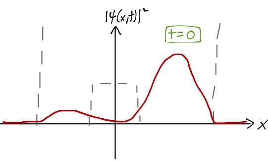
Let's take our initial state to be localized in the right well:
\[ \begin{aligned} \ket{\psi(t=0)} = \frac{1}{\sqrt{2}} \left[ \ket{\psi_{e,1}} + \ket{\psi_{o,1}} \right] \end{aligned} \]
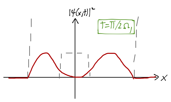
Unlike the infinite-barrier case, the even and odd wavefunctions aren't equal and opposite in the left well, partly due to the energy difference; so this state is only mostly localized in the right well, as we see from plotting \( |\psi(x)|^2 \).
Since we've already written our state vector as a sum over energy eigenstates, it's easy to find the time-evolved state:
\[ \begin{aligned} \ket{\psi(t)} = \frac{1}{\sqrt{2}} \left[ e^{-iE_{e,1} t/\hbar} \ket{\psi_{e,1}} + e^{-iE_{o,1} t/\hbar} \ket{\psi_{o,1}} \right] \\ = \frac{1}{\sqrt{2}} e^{-i(E_{e,1} + E_{o,1})t/(2\hbar)} \left[ e^{i\Omega_1 t/2} \ket{\psi_{e,1}} + e^{-i\Omega_1 t/2} \ket{\psi_{o,1}} \right] \end{aligned} \]
where I have defined the quantity
\[ \begin{aligned} \Omega_1 = \frac{E_{o,1} - E_{e,1}}{\hbar}. \end{aligned} \]
To find the probability density over time, we take the modulus squared, canceling the overall phase in front and giving us
\[ \begin{aligned} |\psi(x,t)|^2 = |\sprod{x}{\psi(t)}|^2 = \frac{1}{2} \left( \psi_{e,1}^2 + \psi_{o,1}^2 \right) + \cos (\Omega_1 t) \psi_{e,1}(x) \psi_{o,1}(x). \end{aligned} \]
where I've simplified knowing that the parity-eigenstate wavefunctions here are real-valued. The effect of the cosine term is that the wavefunction rotates from \( (\psi_{e,1}(x) + \psi_{o,1}(x)) \) at \( t=0 \), to \( (\psi_{e,1}(x) - \psi_{o,1}(x)) \) at \( t=\pi / \Omega_1 \) - at which point the wavefunction is localized in the left well.
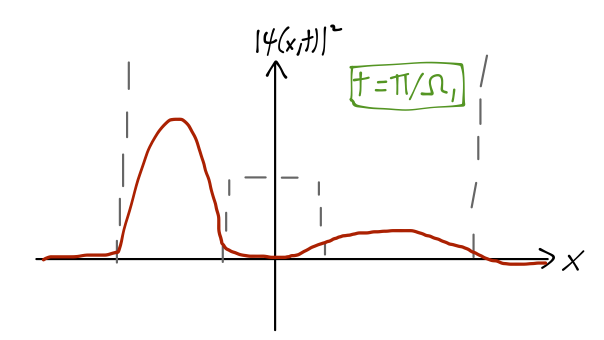
So as the system evolves in time, the position \( x \) shifts from localized in the right well, to the left well and back again with frequency \( f=\Omega_1 / (2\pi) \). Remembering that \( x \) is the distance between the nitrogen atom and the plane of the three hydrogen atoms, and the two potential wells correspond to the two possible orientations of the nitrogen atom, we can see that this motion is exactly the inversion we were looking for. As we've observed, the energy difference \( E_{o,1} - E_{e,1} \) which determines the inversion frequency is very small, as promised; experimentally, it corresponds to the emission of microwave light.
It's interesting to think more about the splitting induced by the finite central barrier. Not only did we find separate energies for even and odd parity eigenstates, but the correction to the even-parity state is negative: \( E_{e,1} < E_1 \). Thus the ground state of the ammonia molecule is actually more stable than we would have predicted if we were ignoring the possibility of inversion. The stability is associated with the fact that the most stable configuration is not one of the individual minima of the potential, corresponding to the nitrogen being oriented in one direction or another, but rather a quantum superposition of both orientations, symmetrically in this case.
There are plenty of examples of this phenomenon in quantum mechanics; I'll give you two famous ones. Another interesting molecule is benzene, \( C_6 H_6 \). The most stable configuration of this molecule is for the six carbon atoms to form a hexagon; this is confirmed by experiment. Since carbon has four valence electrons, every \( C \) should have one bond with a hydrogen atom and three with its carbon neighbors, which means that three of the six sides of the hexagon should be double bonds. It turns out that there are two degenerate configurations with minimum energy:
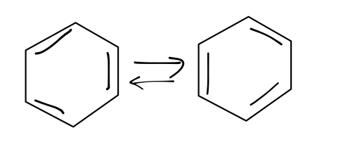
Similar to the inversion of ammonia, it's possible for benzene to invert between these two configurations. The resulting ground state is more stable than either individual state, and is again a superposition of both possibilities.
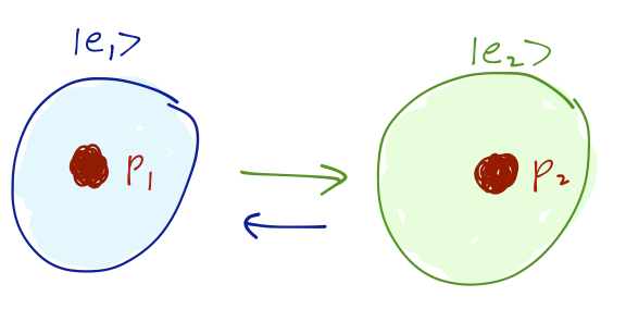
Another good example is given by a much simpler molecule, \( H_2^+ \); two protons with a single electron orbiting them. Again, if the separation between the protons is very large, we find two configurations of the system with equal energy with the electron localized around one proton or the other, giving a ground-state hydrogen atom. However, as a function of the separation the electron will be able to tunnel from one proton to the other, and the most stable configuration is a superposition. The energy of the combined state is again lower than either individual configuration; this is the source of the molecular bond!
(I've given my attempt at describing this phenomenon, but I can't possibly beat Richard Feynman, so if you'd like to recommend more I recommend reading the explanation in his words.)
The two-state description
We can learn more about the inversion of ammonia by isolating the two energy eigenstates \( E_{e,1} \) and \( E_{o,1} \) and treating them as a two-state system, ignoring all of the other states. Let's take as a basis the two states \( \ket{\psi_L^1} \) and \( \ket{\psi_R^1} \) which correspond to a localized particle in the left or right well, respectively. Since we're only considering two states, the entire Hilbert space is spanned by these two kets.
(For the more mathematically inclined, I'll warn you that what we're about to do is phenomenology; we will use what we learned in our wave mechanics example to describe the two-state system of the lowest inversion states. The rigorous justification for doing this will have to wait until we study perturbation theory, but for now you'll just have to accept that we can ignore the other eigenstates because they're relatively well-separated in energy.)
Now we can go back through the steps that we did for the full Schrödinger equation. If we begin with an infinite potential barrier, then the two basis states are orthogonal and have the same energy \( E_1 \). The Hamiltonian matrix is therefore just
\[ \begin{aligned} \hat{H}_0 = \left(\begin{array}{cc} E_1 & 0 \\ 0 & E_1 \end{array} \right). \end{aligned} \]
When the barrier was lowered to \( V_0 \), we noted that the states \( \ket{\psi_L^1} \) and \( \ket{\psi_R^1} \) were no longer orthogonal to each other; a particle localized in one well has a finite probability of being transmitted through the barrier to the other well. This means that in the presence of a finite barrier, our two-state Hamiltonian in this basis can't be diagonal. So we must now have
\[ \begin{aligned} \hat{H} = \left( \begin{array}{cc} E_1 & -A \\ -A & E_1 \end{array} \right) \end{aligned} \]
with \( A>0 \). The fact that the off-diagonal entry \( A \) is real is guaranteed by parity (this is a simple exercise using the definition of parity and the Hermiticity of \( \hat{H} \).) As for the sign of \( A \), the difference is phenomenological: the sign dictates whether the even-parity or odd-parity states are lighter. There is no right answer in general, but we know for this problem that the even-parity states are lighter, giving the structure here.
We've already solved the most general two-state Hamiltonian, which I'll remind you of since it's worth memorizing: given a Hamiltonian
\[ \begin{aligned} \hat{H} = \left( \begin{array}{cc} \epsilon_1 & \delta \\ \delta^\star & \epsilon_2 \end{array} \right) \end{aligned} \]
the energy eigenvalues are
\[ \begin{aligned} E_{\pm} = \frac{\epsilon_1 + \epsilon_2}{2} \pm \sqrt{\left(\frac{\epsilon_1 - \epsilon_2}{2} \right)^2 + |\delta|^2} \end{aligned} \]
and the eigenkets are determined by the mixing matrix
\[ \begin{aligned} \left( \begin{array}{cc} \cos \theta & \sin \theta (\delta^\star/|\delta|) \\ -\sin \theta (\delta/|\delta|) & \cos \theta \end{array} \right) \end{aligned} \]
acting on the initial basis. (You may recognize this as a standard rotation matrix.) Finally, the mixing angle is given by
\[ \begin{aligned} \tan 2\theta = \frac{2|\delta|}{\epsilon_1 - \epsilon_2}. \end{aligned} \]
We see that having \( \epsilon_1 = \epsilon_2 \) and \( \delta \) real makes things particularly simple: since \( \tan 2\theta \) is infinite, we have \( \theta = \pi/4 \), giving the maximally-mixed eigenstates
\[ \begin{aligned} \ket{+} = \frac{1}{\sqrt{2}} (\ket{\psi_L^1} - \ket{\psi_R^1}) = \ket{\psi_o^1} \\ \ket{-} = \frac{1}{\sqrt{2}} (\ket{\psi_L^1} + \ket{\psi_R^1}) = \ket{\psi_e^1}, \end{aligned} \]
and the energy eigenvalues are
\[ \begin{aligned} E_{\pm} = E_1 \pm A. \end{aligned} \]
(Don't forget the minus sign in the mixing matrix! Even though \( \delta = -A \) is real, we still have \( \delta^\star / |\delta| = -A/A = -1 \).)
This reproduces exactly the results we found with our more detailed analysis; namely, that lowering the central potential barrier causes the degeneracy between the energies to be split, and the new energy eigenstates are symmetric and antisymmetric combinations of the single-well states, with the symmetric state having lower energy.
Last time: we reduced the problem of ammonia inversion to studying a two-state system, with Hamiltonian
\[ \begin{aligned} \hat{H} = \left( \begin{array}{cc} E_1 & -A \\ -A & E_1 \end{array} \right). \end{aligned} \]
This was seen to reproduce exactly the results we found with our more detailed analysis; namely, that lowering the central potential barrier causes the degeneracy between the energies to be split, and the new energy eigenstates are symmetric and antisymmetric combinations of the single-well states, with the symmetric state having lower energy. We also find the same time evolution: if we start in the same initial state
\[ \begin{aligned} \ket{\psi(t=0)} = \ket{\psi_R^1} = \frac{1}{\sqrt{2}} [\ket{\psi_e^1} + \ket{\psi_o^1}] \end{aligned} \]
then the time-evolved state is
\[ \begin{aligned} \ket{\psi(t)} = \frac{1}{\sqrt{2}} e^{-iE_1 t/\hbar} [e^{iAt/\hbar} \ket{\psi_e^1} + e^{-iAt/\hbar} \ket{\psi_o^1} \\ = e^{-iE_1t/\hbar} \left[ \cos \left( \frac{At}{\hbar} \right) \ket{\psi_R^1} + i \sin \left( \frac{At}{\hbar} \right) \ket{\psi_L^1} \right]. \end{aligned} \]
So we see inversion between the two local states once again, and can identify the inversion angular frequency \( \Omega_1 = 2A/\hbar \).