Last time: we reduced the problem of ammonia inversion to studying a two-state system, with Hamiltonian
\[ \begin{aligned} \hat{H} = \left( \begin{array}{cc} E_1 & -A \\ -A & E_1 \end{array} \right). \end{aligned} \]
This was seen to reproduce exactly the results we found with our more detailed analysis; namely, that lowering the central potential barrier causes the degeneracy between the energies to be split, and the new energy eigenstates are symmetric and antisymmetric combinations of the single-well states, with the symmetric state having lower energy. We also find the same time evolution: if we start in the same initial state
\[ \begin{aligned} \ket{\psi(t=0)} = \ket{\psi_R^1} = \frac{1}{\sqrt{2}} [\ket{\psi_e^1} + \ket{\psi_o^1}] \end{aligned} \]
then the time-evolved state is
\[ \begin{aligned} \ket{\psi(t)} = \frac{1}{\sqrt{2}} e^{-iE_1 t/\hbar} [e^{iAt/\hbar} \ket{\psi_e^1} + e^{-iAt/\hbar} \ket{\psi_o^1} \\ = e^{-iE_1t/\hbar} \left[ \cos \left( \frac{At}{\hbar} \right) \ket{\psi_R^1} + i \sin \left( \frac{At}{\hbar} \right) \ket{\psi_L^1} \right]. \end{aligned} \]
So we see inversion between the two local states once again, and can identify the inversion angular frequency \( \Omega_1 = 2A/\hbar \).
Ammonia in an electric field
We can make things a little more interesting by adding an external electric field \( \mathcal{E} \) to our two-state system. When the nitrogen atom is localized on one side or another of the hydrogens, it gives the molecule a net electric dipole moment, which can be expressed as an operator,
\[ \begin{aligned} \hat{D} = \left( \begin{array}{cc} -\mu & 0 \\ 0 & \mu \end{array} \right). \end{aligned} \]
I'll remind you that the classical electric dipole moment (EDM) is just the average of the charge density times the displacement, e.g. for point charges
\[ \begin{aligned} \vec{D} = \sum_i q_i \vec{x}_i. \end{aligned} \]
Clearly for ammonia this tells us that the EDM should be equal and opposite in the two inverted configurations, hence the form of the operator above.
The interaction of the ammonia electric dipole with an applied electric field has the Hamiltonian \( \hat{H}_{ED} = \mathcal{E} \hat{D} \). (For simplicity I'm assuming the electric field is aligned with the axis of the molecule.) Thus, the total Hamiltonian of the system is now
\[ \begin{aligned} \hat{H} = \left( \begin{array}{cc} E_1 - \mu \mathcal{E} & -A \\ -A & E_1 + \mu \mathcal{E} \end{array} \right), \end{aligned} \]
giving the energy eigenvalues
\[ \begin{aligned} E_\pm = E_1 \pm \sqrt{A^2 + \mu^2 \mathcal{E}^2} \end{aligned} \]
and the mixing angle is now \( \tan 2\theta = A / (\mu \mathcal{E}) \). When \( \mathcal{E} \gg A \), the energy varies linearly with \( \mathcal{E} \), and the eigenstates become localized to \( \ket{\psi_L^1} \) or \( \ket{\psi_R^1} \); the applied external field pulls the nitrogen to one side or the other. If we plot the energies versus the applied field, we see the expected avoided level crossing; the finite barrier for the two localized states to tunnel into one another, represented by interaction \( A \), breaks the would-be degeneracy at \( \mathcal{E} = 0 \).
It's interesting to calculate the expectation values of the electric dipole moment itself in the two energy eigenstates. It's straightforward to show that
\[ \begin{aligned} \bra{\psi_e^1} \hat{D} \ket{\psi_e^1} = - \bra{\psi_o^1} \hat{D} \ket{\psi_o^1} = \mu \cos (2\theta) = -\frac{\mu^2 \mathcal{E}}{\sqrt{A^2 + \mu^2 \mathcal{E}^2}}. \end{aligned} \]
The ammonia molecule thus has only an induced electric dipole moment; if the external field vanishes, then so does \( \ev{D} \). This is because the energy eigenstates correspond to (anti-)symmetric combinations of the single-well wavefunctions, so that the nitrogen atom has an equal probability of being on either side of the hydrogens, giving zero net dipole moment.
The vanishing of the permanent EDM of the parity eigenstates is actually an example of a very general statement based on parity. Let's step back from our example for a moment and suppose that we have any two parity eigenstates, \( \ket{\alpha} \) and \( \ket{\beta} \):
\[ \begin{aligned} \hat{P} \ket{\alpha} = \epsilon_\alpha \ket{\alpha} \\ \hat{P} \ket{\beta} = \epsilon_\beta \ket{\beta} \end{aligned} \]
where as we know the eigenvalues are \( \epsilon_\alpha, \epsilon_\beta = \pm 1 \). We saw that certain operators have definite properties under parity transformation, in particular the position operator is odd,
\[ \begin{aligned} \hat{P} \hat{x} \hat{P}{}^{-1} = -\hat{x}. \end{aligned} \]
The matrix element of \( \hat{x} \) with respect to the two parity eigenstates is thus
\[ \begin{aligned} \bra{\beta} \hat{x} \ket{\alpha} = \bra{\beta} (\hat{P}^{-1} \hat{P}) \hat{x} (\hat{P}^{-1} \hat{P}) \ket{\alpha} \\ = \epsilon_\alpha \epsilon_\beta (-\bra{\beta} \hat{x} \ket{\alpha}). \end{aligned} \]
Therefore, if the two states have the same parity \( \epsilon_\alpha = \epsilon_\beta \), then we find
\[ \begin{aligned} \bra{\beta} \hat{x} \ket{\alpha} = 0. \end{aligned} \]
This is a specific example of a selection rule. The name comes from application to systems such as transitions between atomic levels, where the atom will "select" only certain possible transition outcomes. In general, a selection rule is a statement that certain matrix elements must vanish based on symmetry considerations.
To tie back to our discussion, as we noted the dipole moment of a charge distribution is linearly propotional to \( \hat{\vec{x}} \), which means that it is also odd under parity. Since many atomic transitions involve electric dipole moments (as we will see later on), this statement for \( \hat{\vec{x}} \) is a direct constraint on radiative transitions in atoms. We can also observe that for any parity eigenstate, we always have
\[ \begin{aligned} \bra{\alpha} \hat{x} \ket{\alpha} = 0. \end{aligned} \]
Thus for any system in which the Hamiltonian is parity invariant, all of the non-degenerate energy eigenstates satisfy this equation, and so they cannot possess any permanent EDM (as is the case for our two-state ammonia example.)
In practice, the electric field \( \mathcal{E} \) will be fairly weak, such that \( \mu \mathcal{E} \ll A \), which means that we can expand to find
\[ \begin{aligned} E_+ = E_{o,1} \approx E_1 + A + \frac{\mu^2 \mathcal{E}^2}{2A}, \\ E_- = E_{e,1} \approx E_1 - A - \frac{\mu^2 \mathcal{E}^2}{2A}. \end{aligned} \]
Once again, we see that where a particle with a static dipole moment would have energy proportional to \( \mathcal{E} \), the ammonia molecule has energy proportional to \( \mathcal{E}^2 \). The coefficient \( \mu^2 / 2A \) is known as the polarizability of our molecule, and it determines how strongly it responds to application of an external electric field. The physical picture you should have here is that while an ordinary dipole moment corresponds to a distribution of charge which is asymmetric in some way, polarizability only requires some sort of free charge distribution to be present; these charges are "pulled apart" by the external field when it is applied.
The force felt by the ammonia molecule in the presence of a field with a spatial gradient is proportional to the gradient of the polarizability,
\[ \begin{aligned} \vec{F} = \frac{\mu^2}{2A} \nabla (\mathcal{E}^2). \end{aligned} \]
It so happens that \( A \) is relatively small for ammonia, which means that (compared to many other molecules) ammonia is quite sensitive to applied electric fields.
We can make use of this interaction to build a Stern-Gerlach-like beam splitter, which will separate the \( \ket{\psi_e^1} \) and \( \ket{\psi_o^1} \) states spatially. This is the first step in constructing an ammonia maser. If we can isolate a beam of molecules in the higher-energy \( \ket{\psi_o^1} \) state, then we pass the beam through a cavity which has an electromagnetic field oscillating at exactly the right frequency in time, all of the excited-state ammonia molecules can be induced to transition back to the lower state with probability 1 in the time it takes to traverse the cavity. As a result, the excess (microwave-frequency) energy is emitted into the cavity, converting molecular energy into the energy of an external electromagnetic field, and thus microwave light.
(Practically, the efficiency will be much lower than 100%; even if we prepare a pure initial state, the molecules will have a distribution of velocities, and so we won't be able to reliably induce the transition inside the cavity. There are much more practical ways of making lasers, but we'll come back to those when we study time-dependent electromagnetic interactions later.)
Example 5: the linear potential well
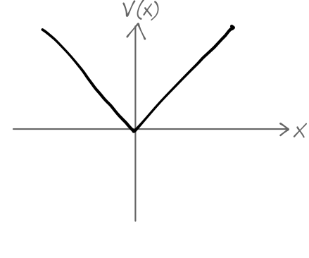
With a thorough understanding of solving the Schrödinger equation in piecewise-constant potentials, we're now ready to tackle a more interesting example: the linear potential,
\[ \begin{aligned} V(x) = k |x|. \end{aligned} \]
Once again, I'll emphasize that this isn't just a randomly chosen example. Like the constant step potential, having a good understanding of linear potential will allow us to obtain good approximations for more complicated potentials which vary "slowly" in \( x \), a definition which we'll make more rigorous shortly. (This will be the formalism of the WKB approximation, which you may have seen before at some level.)
Plugging in our potential, the Schrödinger equation for the energy eigenfunctions becomes
\[ \begin{aligned} -\frac{\hbar^2}{2m} \frac{d^2 u_E}{dx^2} + k|x| u_E(x) = E u_E(x) \end{aligned} \]
where I'm following Sakurai's notation and using \( u_E(x) \) instead of \( \psi_E(x) \) for the eigenfunctions. Since \( V(-x) = V(x) \), we see that parity is a good symmetry of our system again, so we can focus on \( x>0 \) and look for eigenfunctions with definite parity.
We can start by making our lives easier and scaling out all of the dimensionful quantities in this equation. Defining some arbitrary length scale \( x_0 \), we can divide through to find (again, now with \( x>0 \) fixed)
\[ \begin{aligned} -\frac{\hbar^2}{2mkx_0} \frac{d^2 u_E}{dx^2} + \frac{x}{x_0} u_E(x) = \frac{E}{kx_0} u_E(x) \\ -\frac{\hbar^2}{2mkx_0^3} \frac{d^2 u_E}{dy^2} + y u_E(y) = \frac{E}{kx_0} u_E(y) \end{aligned} \]
where I've defined \( y=x/x_0 \). It's now clear that we can maximally simplify things by choosing
\[ \begin{aligned} x_0 = \left(\frac{\hbar^2}{mk}\right)^{1/3}. \end{aligned} \]
Letting \( \epsilon \equiv E / kx_0 \), then we arrive at the simplified equation
\[ \begin{aligned} \frac{d^2 u_E}{dy^2} - 2(y-\epsilon) u_E(y) = 0. \end{aligned} \]
It's interesting to note that \( y = \epsilon \) implies that \( x/x_0 = E / (kx_0) \), or \( x = E/k \), which is in fact the classical turning point. We can simplify one more time by defining a new variable \( z \) proportional to the distance from the turning point, \( z = 2^{1/3} (y-\epsilon) \), giving us
\[ \begin{aligned} \frac{d^2 u_E}{dz^2} - z u_E(z) = 0. \end{aligned} \]
This is now in standard form for a well-known differential equation, known as the Airy equation; its solutions are the Airy functions \( {\rm Ai}(z) \). The Airy function has an interesting functional form: for \( z < 0\ \) it oscillates somewhat like a plane wave, while for \( z > 0\ \) it is damped to zero somewhat like a pure exponential. Since the classical turning point is exactly where the energy crosses the potential barrier, this is exactly the behavior we expect.
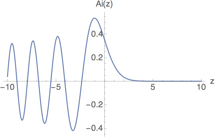
(In fact, as a second-order equation it should have two solutions; there is a second set of Airy functions denoted \( {\rm Bi}(x) \). You can probably guess that these also look like oscillatory solutions going over to exponential; the important difference is that \( {\rm Bi}(x) \) goes to infinity as \( x \rightarrow \infty \), which means it violates our boundary conditions for this particular problem.)
Now we have to remember that we've ignored \( x<0 \) because we're supposed to be looking for parity eigenstates. If our solution has even parity, then we have the condition
\[ \begin{aligned} u_E(-x) = +u_E(x). \end{aligned} \]
If we take \( x \) to be some infinitesmal value \( \epsilon \), then this implies that \( u_E(-\epsilon) - u_E(\epsilon) = 0 \), which in the limit \( \epsilon \rightarrow 0 \) tells us that \( u_E'(0) = 0 \). On the other hand, for the odd solutions \( u_E(-x) = -u_E(x) \) we can simply plug in \( x=0 \) to find that \( u_E(0) = 0 \). Thus, our expected quantization condition that the energy eigenstates must satisfy is either \( {\rm Ai}(z) = 0 \) or \( {\rm Ai}'(z) = 0 \). Unraveling our string of definitions above, if we find a root at \( z_0 \) then the corresponding bound-state energy is
\[ \begin{aligned} E = -z_0 (kx_0) / 2^{1/3} = -(z_0 / 2^{1/3}) (\hbar^2 k^2/m)^{1/3}. \end{aligned} \]
There are real physical systems which having linear potential energies; a quantum system subject to gravity is one example, which we'll return to. The strong nuclear force which binds protons and neutrons together is another example; the potential energy between quarks is approximately linear as the separation between them becomes large. Our simple solution here actually gives quite a reasonable description for the energy spectrum of quark-antiquark bound states, known as quarkonium. The constant \( k \) can be determined from the observed spectrum, and is about \( 1.6 \times 10^5 \) N, corresponding to a gravitational force of 16 tons; the strong force is strong indeed!