The solution to the linear potential actually has a much broader set of applications, as part of an approximation method known as the WKB approximation, after its inventors Wentzel, Kramers, and Brillouin. Start by writing down Schrödinger's equation in one dimension with some arbitrary potential:
\[ \begin{aligned} \frac{d^2 u_E}{dx^2} + \frac{2m}{\hbar^2} (E-V(x)) u_E(x) = 0. \end{aligned} \]
If \( V(x) \) is constant, then we've seen that we can easily find solutions as complex exponentials, with the wave number determined by the difference \( E-V \). What if we define a more general version of the wave number that depends on \( x \)?
\[ \begin{aligned} k(x) = \left[ \frac{2m}{\hbar^2} (E-V(x)) \right]^{1/2} \\ \kappa(x) = \left[ \frac{2m}{\hbar^2} (V(x)-E) \right]^{1/2} \end{aligned} \]
where \( k(x) = -i \kappa(x) \), but as usual we prefer to work with real wave numbers. Then the Schrödinger equation can be written simply as
\[ \begin{aligned} \frac{d^2 u_E}{dx^2} + [k(x)]^2 u_E(x) = 0. \end{aligned} \]
As we know, if \( k(x) \) is constant then the solutions are exponentials, \( e^{\pm ikx} \). Does a solution of exponential form, but with some additional \( x \) dependence, always work? We can try the ansatz
\[ \begin{aligned} u_E(x) = \exp \left[ i W(x) / \hbar \right] \end{aligned} \]
in which case, the Schrödinger equation is transformed to an equation for \( W(x) \),
\[ \begin{aligned} i \hbar \frac{d^2 W}{dx^2} - \left( \frac{dW}{dx} \right)^2 + [p(x)]^2 = 0. \end{aligned} \]
(Note that I've rewritten \( p(x) = \hbar k(x) \).) This is a messy equation, which we can't hope to solve in general. We can think back to the case which we could solve, with constant potential and therefore \( W(x) = \hbar kx \), which trivially gives us back \( p(x) = \hbar k \) since the second derivative vanishes. In fact, you can see that if the second-derivative term vanishes in general, we can solve for \( W(x) \) simply by integrating the wave number \( k(x) \). We will find that the validity of what we're about to do assumes the "slow variation" of the wavefunction,
\[ \begin{aligned} \hbar \left| \frac{d^2 W}{dx^2} \right| \ll \left| \frac{dW}{dx} \right|^2. \end{aligned} \]
You should suspect that this has something to do with the semi-classical (small \( \hbar \)) limit, since if \( \hbar \rightarrow 0 \) the condition is always true. This is also why I'm working with \( p(x) \) and not \( k(x) \); we're dealing with solutions that are oscillating exponentials, which means that when we say the potential is "slowly varying" we mean compared to the de Broglie wavelength \( \lambda = 2\pi \hbar / p \). Trying to keep the wave number \( k \) fixed while varying \( \hbar \) isn't a sensible way to take the limit.
Let's come back to validity after we find our solution. Now in the semiclassical spirit, let's assume that we can write our solution for \( W(x) \) as a power series in \( \hbar \):
\[ \begin{aligned} W(x) = W_0(x) + \hbar W_1(x) + \hbar^2 W_2(x) + ... \end{aligned} \]
(Beware: if you have read the derivation in Sakurai, he has secretly done this and then recombined terms, so his \( W_1(x) \) is equal to my \( W_0(x) + \hbar W_1(x) \). Shankar and other textbooks give a more standard derivation.) Returning to our differential equation above and plugging in, then keeping only the first few terms in the expansion we find
\[ \begin{aligned} \left[ - W_0'(x)^2 + p(x)^2 \right] \hbar^0 + \left[ i W_0''(x) - 2 W_0'(x) W_1'(x) \right] \hbar + \mathcal{O}(\hbar^2) = 0. \end{aligned} \]
So at leading order in \( \hbar \), dropping the second term, we find that we just have to integrate to find our approximate solution,
\[ \begin{aligned} W_0'(x) = \pm p(x) \end{aligned} \]
and then \( W_0(x) \) is simply given by integral \( \int dx\ \hbar k(x) \). We can do better than this, however; the next term is still not too bad to work with. At order \( \hbar \) both expressions must vanish, so we still have \( W_0'(x) = p(x) \), and therefore
\[ \begin{aligned} W_0''(x) = p'(x). \end{aligned} \]
Solving the second expression for \( W_1'(x) \) then yields
\[ \begin{aligned} -2i W_1'(x) = \frac{W_0''(x)}{W_0'(x)} = \frac{p'(x)}{p(x)} \end{aligned} \]
or integrating both sides,
\[ \begin{aligned} -2i W_1(x) = \log p(x) + C \\ \Rightarrow W_1(x) = i \log \sqrt{p(x)} + C'. \end{aligned} \]
Putting our two solutions back together and integrating, we have
\[ \begin{aligned} u_E(x) \approx \frac{1}{\sqrt{p(x)}} \exp \left[ \pm \frac{i}{\hbar} \int^x dx'\ p(x') \right] \\ = \frac{1}{\sqrt{2m(E-V(x))}} \exp \left[ \pm \frac{i}{\hbar} \int^x dx' \sqrt{2m(E-V(x'))} \right], \end{aligned} \]
reintroducing the position-dependent wave number \( k(x) = \sqrt{2m(E-V(x))}/\hbar \). As usual, there are two solutions, and the most general solution to the differential equation is a linear combination with arbitrary coefficients. Here we've assumed that \( E > V(x) \); if the opposite is true, then we switch to \( \kappa(x) \) and flip the sign under the square root as usual. Thus, the most general WKB solution can be written in the form
\[ \begin{aligned} u_E(x) \approx \begin{cases} \frac{1}{\sqrt{k(x)}} \exp \left[ \pm i \int^x dx' k(x') \right],& E > V(x); \\ \frac{1}{\sqrt{\kappa(x)}} \exp \left[ \pm \int^x dx' \kappa(x') \right],& E < V(x). \end{cases} \end{aligned} \]
The funny-looking limit on this integral is a reminder that we don't care about the overall normalization of this solution, since it's multiplied by an arbitrary constant; we can pick any limit we want as long as we're consistent.
What we've done here is a truncation: we're ignoring all of the higher-order terms \( W_2(x), W_3(x), ... \) on the assumption that they are "small" (linked to the idea that in some sense \( \hbar \) is "small".) If we've made a good assumption, then our series should be converging rapidly to the correct solution, i.e. we should find that
\[ \begin{aligned} \hbar W_1(x) \ll W_0(x). \\ i \hbar \log \sqrt{p(x)} \ll \int^x dx' p(x') \\ i \hbar \int^x dx' \frac{p'(x')}{p(x')} \ll \int^x dx' p(x'). \end{aligned} \]
Since we're doing the same integral on both sides, the inequality will thus be satisfied as long as
\[ \begin{aligned} |k'(x)| \ll |k(x)^2| \end{aligned} \]
(where the absolute value lets us deal with the \( E < V(x) \) case in a compact way.) We can interpret this condition physically by defining a position-dependent de Broglie wavelength,
\[ \begin{aligned} \lambda(x) \equiv \frac{2\pi}{k(x)}. \end{aligned} \]
Since
\[ \begin{aligned} \lambda'(x) = -\frac{2\pi k'(x)}{k(x)^2}, \end{aligned} \]
we can see that our consistency condition for the WKB approximation is just that
\[ \begin{aligned} \left| \frac{d\lambda}{dx} \right| \ll 1 \end{aligned} \]
(ignoring the constant factors.) This can be usefully rewritten by noting that
\[ \begin{aligned} \lambda'(x) = -\lambda(x) \frac{p'(x)}{p(x)} \\ p'(x) = \frac{V'(x)}{2\sqrt{2m(E-V(x))}} = \frac{V'(x)}{p(x)} \end{aligned} \]
and so the condition becomes
\[ \begin{aligned} \lambda(x) \left| \frac{dV}{dx} \right| \ll \frac{[p(x)]^2}{m}. \end{aligned} \]
Thus, WKB is valid when the potential energy is changing slowly (in units of the local wavelength), compared to the kinetic energy.
WKB connection formulas
The consistency conditions can always be violated by a rapidly changing \( V(x) \), but we are guaranteed to run into trouble at the classical turning points, where \( V = E \) causes \( k(x) \) to vanish, leading to a rapidly diverging wavelength. Thus, if we try to apply the WKB approximation to an arbitrary potential, we will have gaps in our solution wherever \( V(x) \approx E \). Fortunately, when this latter condition is satisfied we can come up with another approximate solution to the Schrödinger equation, and we can then write down a complete solution by patching WKB wavefunctions together.
If we make the (usually justified) assumption that the function \( V(x) - E \) has a single zero at \( x_0 \), then a Taylor expansion gives
\[ \begin{aligned} V(x) - E \approx C(x-x_0) \end{aligned} \]
and the Schrödinger equation becomes
\[ \begin{aligned} -\frac{\hbar^2}{2m} \frac{d^2 u_E}{dx^2} + C(x-x_0) u_E(x) = 0. \end{aligned} \]
We solved this equation last time; it's the same equation for a particle in a linear potential well, so we know that the solutions are Airy functions. Since we are trying to join together WKB solutions on either side of a turning point, we expect to transition from oscillatory behavior to exponential growth and decay, or vice-versa; the Airy functions, as we've seen, smoothly interpolate from one to the other. In fact, the asymptotic forms of the Airy function are well known:
\[ \begin{aligned} (z \rightarrow +\infty): {\rm Ai}(z) \rightarrow \frac{1}{2\sqrt{\pi}} z^{-1/4} \exp \left( -\frac{2}{3} z^{3/2} \right) \\ (z \rightarrow -\infty): {\rm Ai}(z) \rightarrow \frac{1}{\sqrt{\pi}} |z|^{-1/4} \cos \left( \frac{2}{3} |z|^{3/2} - \frac{\pi}{4} \right). \\ \end{aligned} \]
These asymptotic forms are precisely what the WKB solutions look like (even down to the \( z^{-1/4} \sim 1/\sqrt{k} \).) Matching the WKB solutions onto the joining functions at the boundaries gives rise to a set of "connection formulas", which work just like any other set of boundary conditions, allowing us to determine the arbitrary constants in our general solution.
I'll skip the details of the derivation, and just give you the results for the connection formulas. If we have a potential \( V(x) \) with a classical turning point at \( x=a \), and assume that \( V'(a) > 0 \):
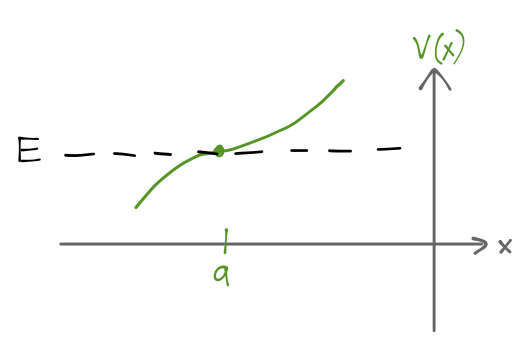
then if for \( x > a \) we have the general WKB solution
\[ \begin{aligned} \frac{A}{\sqrt{\kappa(x)}} \exp \left[ -\int_a^x dx'\ \kappa(x') \right] + \frac{B}{\sqrt{\kappa(x)}} \exp \left[ \int_a^x dx'\ \kappa(x') \right], \end{aligned} \]
then the solution for \( x < a \) takes the form
\[ \begin{aligned} \frac{2A}{\sqrt{k(x)}} \cos \left[ \int_x^a dx' k(x') - \frac{\pi}{4} \right] - \frac{B}{\sqrt{k(x)}} \sin \left[ \int_x^a dx' k(x') - \frac{\pi}{4} \right]. \end{aligned} \]
If instead the potential is decreasing at \( a \), then we have exponentials on the left and oscillation on the right. The connection formulas are exactly the same, but with the replacement \( x-a \rightarrow a-x \) (which just flips the limits of integration upside down everywhere.)