First, a brief note on WKB approximation and using the asymptotic form of the Airy functions. A natural question is whether it's consistent to assume that the asymptotic forms are good replacements when we're doing WKB, or whether this is secretly an additional assumption. Recall that the condition for WKB to work is
\[ \begin{aligned} |k'(x)| \ll |k^2(x)|. \end{aligned} \]
In the vicinity of a linear potential region, i.e. if \( V(x) - E \approx g(x-a) \) where \( g \) is a constant, the solutions to the Schrödinger equation become \( {\rm Ai}(z) \) and \( {\rm Bi}(z) \), where \( z \) is the dimensionless combination
\[ \begin{aligned} z = \left( \frac{2mg}{\hbar^2} \right)^{1/3} (x-a). \end{aligned} \]
In the process of solving for the wavefunction, it's easy to see that \( k^2 \propto -z \), so the WKB condition becomes (roughly) \( |z| \gg 1 \). This is good enough for us to use the asymptotic forms: numerically, the Airy functions become very close to their approximations around \( |z| \sim 3 \) or so. (The asymptotic forms actually diverge at \( z=0 \), whereas the real Airy functions don't; but we're only using them to connect between asymptotic regions, so we don't care what happens at \( z=0 \).)
I skipped quickly through details here; the full discussion can be found in Merzbacher 7.2.
Since we went to all the trouble of introducing WKB in gruesome detail, let's go through a couple of useful applications.
WKB and bound states
Suppose we have a potential well with some shape, and consider a bound state with energy such that the turning points are at \( x=a \) and \( x=b \). We can divide the potential into three regions:
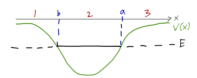
Starting in region 1, as usual the condition that the wavefunction can't blow up as \( x \rightarrow -\infty \) forces us to consider only a single term in the solution,
\[ \begin{aligned} \psi_1(x) \approx \frac{A}{\sqrt{\kappa(x)}} \exp \left[- \int_x^b dx'\ \kappa(x') \right]. \end{aligned} \]
To find the solution to the right of turning point \( b \), we need the WKB connection formula, which I'll reproduce from before:
\[ \begin{aligned} \frac{A}{\sqrt{\kappa(x)}} \exp \left[ -\int_x^b dx'\ \kappa(x') \right] + \frac{B}{\sqrt{\kappa(x)}} \exp \left[ \int_x^b dx'\ \kappa(x') \right] \leftrightarrow \frac{2A}{\sqrt{k(x)}} \cos \left[ \int_b^x dx' k(x') - \frac{\pi}{4} \right] - \frac{B}{\sqrt{k(x)}} \sin \left[ \int_b^x dx' k(x') - \frac{\pi}{4} \right]. \end{aligned} \]
(note that I've substituted in \( b \) as the turning point and I've reversed the integrals from the connection formula written last time.) We thus read off the solution in region 2 as
\[ \begin{aligned} \psi_2(x) \approx \frac{2A}{\sqrt{k(x)}} \cos \left[ \int_b^x dx'\ k(x') - \frac{\pi}{4} \right]. \end{aligned} \]
We can rewrite this in the form
\[ \begin{aligned} \psi_2(x) \approx \frac{2A}{\sqrt{k(x)}} \cos \left[ \int_b^a dx'\ k(x') - \int_x^a dx'\ k(x') - \frac{\pi}{4} \right] \\ = \frac{2A}{\sqrt{k(x)}} \left( \cos \left[ \int_b^a dx'\ k(x') \right] \cos \left[ \int_x^a dx'\ k(x') + \frac{\pi}{4} \right] \right. \\ +\left. \sin \left[ \int_b^a dx'\ k(x') \right] \sin \left[ \int_x^a dx'\ k(x') + \frac{\pi}{4} \right] \right) \\ = (...) \left( -\cos(C) \sin \left[\int_x^a dx' k(x') - \frac{\pi}{4} \right] + \sin(C) \cos \left[ \int_x^a dx' k(x') - \frac{\pi}{4} \right] \right). \end{aligned} \]
This is now in the standard form for the connection formula at the right turning point \( x=a \), which will give us the wavefunction in region 3. However, once again we have to insist that the positive exponential solution vanishes in region 3, to give a normalized wavefunction. By inspection of the connection formula, the positive exponential matches on to the sine solution, which means that the coefficient of the sine must vanish:
\[ \begin{aligned} \cos(C) = \cos \left[ \int_b^a dx'\ k(x') \right] = 0, \end{aligned} \]
or
\[ \begin{aligned} \int_b^a dx'\ k(x') = \left(n + \frac{1}{2}\right) \pi, \end{aligned} \]
or
\[ \begin{aligned} \int_b^a \sqrt{2m(E-V(x))} = \pi \hbar \left(n + \frac{1}{2} \right). \end{aligned} \]
So long as the WKB approximation works well for our chosen potential (which primarily means that the turning points \( a \) and \( b \) must be separated by many wavelengths), this formula tells us what the bound-state energies can be.
We should note that the quantity we are integrating over on the left-hand side is exactly the momentum, \( p(x) = \hbar k(x) \). Furthermore, the two points \( a \) and \( b \) are the classical turning points; a classical particle with energy \( E \) would move in an "orbit" between \( x=a \) and \( x=b \). We can thus rewrite the integral in a more classical way, as an integral over the phase-space trajectory of our particle,
\[ \begin{aligned} \oint p(x) dx = h \left(n + \frac{1}{2} \right) \end{aligned} \]
where now we've recovered the un-barred Planck constant. (Note that we picked up a 2 since the phase-space integral goes around a complete circle, so it's double the integral we started with.) Except for the shift by \( 1/2 \), this is exactly the Bohr-Sommerfeld quantization rule which was one of the foundations of the "old quantum" theory. Whereas a classical particle could have any bound-state energy \( E \), the quantization rule allows only bound states for which the above action integral gives integer multiples of \( h \).
WKB and quantum tunneling
We can also gain some very useful insights from WKB in the case that we have a potential barrier, rather than a well. Again, we assume an arbitrary shape for \( V(x) \), but with slow enough variation that WKB can be applied, and we consider \( E < V_{\rm max} \) so that the particle cannot pass though the barrier classically.
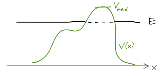
As with the example of the square potential barrier, we can start by writing down our arbitrary solution in the three regions defined by the turning points \( a \) and \( b \):
\[ \begin{aligned} \psi(x) = \begin{cases} \frac{A}{\sqrt{k(x)}} \exp \left[i \int_a^x dx' k(x') \right] + \frac{B}{\sqrt{k(x)}} \exp \left[ -i \int_a^x dx' k(x') \right], & (x < a); \\ \frac{C}{\sqrt{\kappa(x)}} \exp \left[- \int_a^x dx' \kappa(x') \right] + \frac{D}{\sqrt{\kappa(x)}} \exp \left[ \int_a^x dx' \kappa(x') \right], & (a < x < b); \\ \frac{F}{\sqrt{k(x)}} \exp \left[i \int_b^x dx' k(x') \right] + \frac{G}{\sqrt{k(x)}} \exp \left[ -i \int_b^x dx' k(x') \right], & (x > b). \\ \end{cases} \end{aligned} \]
With the connection formulas in hand, we can easily find the relationship between these coefficients. In fact, the result turns out to be quite simple: in matrix form, we find that
\[ \begin{aligned} \left( \begin{array}{c} A \\ B \end{array} \right) = \frac{1}{2} \left( \begin{array}{cc} 2\theta + \frac{1}{2\theta} & i (2\theta - \frac{1}{2\theta}) \\ -i(2\theta - \frac{1}{2\theta}) & 2\theta + \frac{1}{2\theta} \end{array} \right) \left( \begin{array}{c} F \\ G \end{array} \right) \end{aligned} \]
where
\[ \begin{aligned} \theta = \exp \left[ \int_a^b dx' \kappa(x') \right]. \end{aligned} \]
So as far as the transmission and reflection of incoming waves are concerned, all of the information about the barrier is encoded in the single integral which gives \( \theta \). We can read off the transmission coefficient from this matrix,
\[ \begin{aligned} T = \frac{|F|^2}{|A|^2} = \frac{4}{\left(2\theta + \frac{1}{2\theta}\right)^2}. \end{aligned} \]
In the limit that the barrier is high and wide, then \( \theta \) becomes large, and we simply have
\[ \begin{aligned} T \approx \frac{1}{\theta^2} = \exp \left[ -2 \int_a^b dx'\ \kappa(x') \right] = \exp \left[ -\frac{2}{\hbar} \int_a^b \sqrt{2m(V(x)-E)} \right]. \end{aligned} \]
Example: alpha decay
An early quantum-mechanical model of nuclear \( \alpha \) decay is given by the Gamow-Gurney-Condon theory (see here for a historical review), which treats it entirely as a tunneling process. Roughly, the model treats the \( \alpha \) particle (which is a helium-4 nucleus) as a single object which is bound in a deep, square potential well of width \( R \), corresponding to the radius of the parent nucleus. Once the \( \alpha \) particle escapes, it will be repelled by the Coulomb force. So the overall potential looks like this:
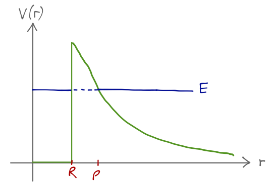
\[ \begin{aligned} V(x) = \begin{cases} 0, & 0 < r < R;\\ \frac{2Ze^2}{r}, & r > R. \end{cases} \end{aligned} \]
where \( Z \) is the charge of the daughter nucleus in the decay. Ignoring the fact that the potential step at \( R \) is pretty sharp and not WKB friendly at all (we'll take \( R \) to be very small anyway, the interesting physics comes from the Coulomb barrier), we can calculate the transmission coefficient in the approximation of a large barrier:
\[ \begin{aligned} -\frac{1}{2} \log T = \int_R^\rho dr'\ r'^2 \kappa(r') = \frac{\sqrt{2m}}{\hbar} \int_R^\rho dr' r'^2 \sqrt{\frac{2Ze^2}{r'} - E}. \end{aligned} \]
(where I've included the \( r'^2 \) in the integration to acknowledge the fact that this is happening in three dimensions, although we're not doing a full treatment yet.)
The position \( \rho \) of the second turning point is given by the condition \( E = 2Ze^2/\rho \). If we take \( E = \frac{1}{2} mv^2 \) using the speed of the escaping alpha, then in the limit \( R \rightarrow 0 \) the integral yields the result
\[ \begin{aligned} -\frac{1}{2} \log T \approx \frac{2\pi Z e^2}{\hbar v} \end{aligned} \]
or
\[ \begin{aligned} T \approx \exp \left[ -\frac{4\pi Z e^2}{\hbar v}\right]. \end{aligned} \]
(If you do the integral properly in Mathematica, you can find a full expression including the \( R \) dependence.) The striking feature here is that the transmission probability is exponentially sensitive to the nuclear charge, \( Z \). We can turn this transmission coefficient into a decay rate: if on average the alpha particle strikes the barrier inside the nucleus with a frequency of \( v/(2R) \), then the decay rate should be
\[ \begin{aligned} \lambda = \frac{Tv}{2R}. \end{aligned} \]
This formula (or more accurately, the full expression with the \( R \) values included) does an excellent job of reproducing experimental data for alpha decay spanning 23 orders of magnitude in lifetime!