In our examples so far, we've frequently invoked symmetry under parity as a constraint on our solutions. This is an example of a discrete symmetry, since the operation of parity reflection is not a continuous change of our system. (The discreteness of \( \hat{P} \) ensures that it has a finite spectrum of eigenvalues, incidentally.)
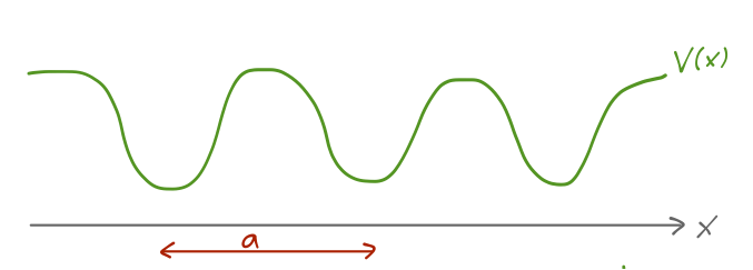
There is another, much more powerful example of a discrete symmetry that we can find in a potential \( V(x) \), which is known as periodicity: in one dimension, it is the condition that
\[ \begin{aligned} V(x \pm a) = V(x) \end{aligned} \]
for some particular length scale \( a \). This is, once again, a discrete symmetry, corresponding to the operation of shifting our entire potential by a finite length \( a \). This operation is known as finite translation or lattice translation (to distinguish it from symmetry under infinitesmal translations by some arbitrary \( \epsilon \).) Obviously, this will be an extremely important symmetry for the description of crystals and other solid-state systems.
Just as we did for parity, we can define a translation operator which will act on our system by performing a finite shift. We define the operator \( \hat{\tau}(L) \), which will act in a straightforward way on position eigenstates:
\[ \begin{aligned} \hat{\tau}(L) \ket{x} = \ket{x+L}. \end{aligned} \]
This tells us that the position operator itself must transform as
\[ \begin{aligned} \hat{\tau}^\dagger(L) \hat{x} \hat{\tau}(L) = \hat{x} + L. \end{aligned} \]
Furthermore, we expect that translation by \( -L \) and then by \( L \) should give back the original state, from which we see that \( \hat{\tau}^{-1}(L) = \hat{\tau}(-L) \). However, we can see that
\[ \begin{aligned} \hat{\tau}^\dagger(-L) \hat{x} \hat{\tau}(-L) = \hat{x} - L \\ \hat{\tau}^\dagger(L) [...] \hat{\tau}(L) = \hat{\tau}^\dagger(L) \hat{x} \hat{\tau}(L) - L \hat{\tau}^\dagger(L) \hat{\tau}(L) \\ = \hat{x} + L (1 - \hat{\tau}^\dagger(L) \hat{\tau}(L)) \end{aligned} \]
which, given the observation that \( \hat{\tau}^{-1}(L) = \hat{\tau}(-L) \), must equal \( \hat{x} \); so we also find that \( \hat{\tau}(L) \) is a unitary operator.
What about the momentum operator?
\[ \begin{aligned} \bra{x'} \hat{\tau}^\dagger(L) \hat{p} \hat{\tau}(L) \ket{x} = \bra{x'+L} \hat{p} \ket{x+L} = \delta((x+L) - (x'+L)) \frac{\hbar}{i} \frac{\partial}{\partial x} \\ = \delta(x - x') \frac{\hbar}{i} \frac{\partial}{\partial x} = \bra{x'} \hat{p} \ket{x} \end{aligned} \]
i.e. finite translation leaves the momentum unchanged (as we might have intuitively guessed.)
Once again, we should emphasize that for a system with lattice translation invariance, translation by an arbitrary length \( L \) will not be a symmetry. However, for the particular operator \( \tau(a) \) such that
\[ \begin{aligned} \hat{\tau}^\dagger(a) V(\hat{x}) \hat{\tau}(a) = V(\hat{x} + a) = V(\hat{x}) \end{aligned} \]
then we find that
\[ \begin{aligned} \hat{\tau}^\dagger(a) \hat{H} \hat{\tau}(a) = \hat{H} \\ \Rightarrow [\hat{H}, \hat{\tau}(a)] = 0. \end{aligned} \]
where the last line follows since \( \hat{\tau}(L) \) is unitary. This commutator guarantees that we will be able to find simultaneous eigenstates of \( \hat{H} \) and \( \hat{\tau}(a) \).
Tight-binding approximation
It's interesting to start with the case of a potential which is periodic, but with infinite potential barriers between neighboring identical wells of width \( a \).
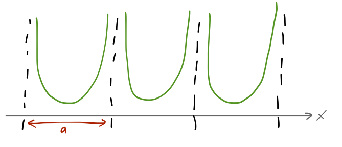
Suppose that if we solved the Schrödinger equation for one copy of this potential, we would find a set of bound states with energies \( E \). Labeling the infinite set of wells by some integers \( n \), we can construct a state \( \ket{n, E} \) which is equal to the \( E \) eigenstate in well \( n \), and zero elsewhere. So \( \hat{H} \ket{n, E} = E \ket{n, E} \), and there are an infinite number of such states in our infinite, periodic potential.
These states, however, are not eigenstates of the lattice translation operator, which clearly acts to give us
\[ \begin{aligned} \hat{\tau}(a) \ket{n, E} = \ket{n+1, E}. \end{aligned} \]
This should all remind you of our treatment of the double-well potential for ammonia; there we similarly constructed localized energy eigenstates in the two wells, but found that they were not parity eigenstates. However, we could take the symmetric and anti-symmetric combinations \( \ket{L} + \ket{R} \) and \( \ket{L} - \ket{R} \) to obtain states which were simultaneously parity and energy eigenstates.
We can do the same thing here, except that because of the way translation acts, any simultaneous eigenstate of \( \hat{H} \) and \( \hat{\tau}(a) \) must be an infinite sum of localized states. In fact, we find that such a state should look like this:
\[ \begin{aligned} \ket{\theta, E} = \sum_{n=-\infty}^\infty e^{in\theta} \ket{n,E}. \end{aligned} \]
Acting with the translation operator, we see that
\[ \begin{aligned} \hat{\tau}(a) \ket{\theta, E} = \sum_{n=-\infty}^\infty e^{in \theta} \ket{n+1, E} \\ = \sum_{n=-\infty}^\infty e^{i(n-1)\theta} \ket{n, E} \\ = e^{-i\theta} \ket{\theta, E}. \end{aligned} \]
So indeed, \( \ket{\theta, E} \) is an eigenstate of lattice translation (and also of \( \hat{H} \), since we constructed it as a sum of energy eigenstates.) The eigenvalue with respect to translation is a pure phase, so we can see that \( \ket{\theta, E} = \ket{\theta+2\pi, E} \) for any \( \theta \). By convention we take the physical state to be labelled by \( -\pi < \theta \leq \pi \).
Bonus material: why a phase?
A very good question came up in class: although the above derivation works just fine, the first step is a little vague. Why should the coefficients of \( \ket{\theta, E} \) be pure phases, instead of just arbitrary complex numbers?
The best way to answer this question (which I didn't want to attempt in real time) is to just try the more general expansion: we allow an arbitrary complex coefficient for each well eigenstate,
\[ \begin{aligned} \ket{T, E} = \sum_{n=-\infty}^\infty z_n \ket{n, E}. \end{aligned} \]
Now what happens if we act with the translation operator? We find the following, doing the same sum redefinition trick:
\[ \begin{aligned} \hat{\tau}(a) \ket{T, E} = \sum_{n=-\infty}^\infty z_{n-1} \ket{n, E}. \end{aligned} \]
In general, there's no reason for this state to be a translation eigenstate. But if we assume it is, then we find the equation
\[ \begin{aligned} \hat{\tau}(a) \ket{T, E} = T \ket{T, E} \\ \sum_{n=-\infty}^\infty z_{n-1} \ket{n,E} = T \sum_{n=-\infty}^\infty z_n \ket{n,E}. \end{aligned} \]
Since both sides are summing over the same states, every coefficient in the sum has to be identical, i.e. we find the result
\[ \begin{aligned} z_{n-1} = T z_n. \end{aligned} \]
This is a significant constraint, but it doesn't prove the \( z_n \) must be a phase yet. We go a step further and apply the identity operator, in the form \( \hat{\tau}^\dagger(a) \hat{\tau}(a) \):
\[ \begin{aligned} \bra{T, E} \hat{\tau}^\dagger(a) \hat{\tau}(a) \ket{T,E} = |T|^2 \end{aligned} \]
since \( \bra{T,E} \hat{\tau}^\dagger(a) = (\hat{\tau}(a) \ket{T,E})^\dagger \). But this is also just \( \sprod{T,E}{T,E} = 1 \), so \( T \) must be a pure phase \( T = e^{i\theta} \), which means that
\[ \begin{aligned} z_n = e^{in\theta} z_0. \end{aligned} \]
So up to an overall constant, the form \( \ket{\theta, E} \) is the only possibility for an eigenstate of \( \hat{\tau}(a) \). The key here is actually a much more general result, which we basically just proved: the eigenvalues of a unitary operator are pure phases.
This is, so far, something of a formal exercise; the construction of the \( \ket{\theta, E} \) states doesn't alter the energy spectrum at all since the wells have infinite barriers between them. At this point we'll focus on a single eigenstate \( E_0 \), and label our well-centered states as \( \ket{n} \). Let's lower the barriers between the wells to be finite, but still high. In fact, we will assume that the barriers are high enough that while tunneling between adjacent wells is possible, leading to overlap of the wavefunctions, the overlap with wells separated by two or more barriers is totally negligible. In other words, the matrix elements of the Hamiltonian between localized states is
\[ \begin{aligned} \bra{n} \hat{H} \ket{n} = E_0 \\ \bra{n'} \hat{H} \ket{n} = -\Delta \delta_{n', n\pm 1}. \end{aligned} \]
This set of assumptions is known in solid state physics as the tight-binding approximation. Now, the localized states in an individual well are no longer energy eigenstates: the action of the Hamiltonian gives us
\[ \begin{aligned} \hat{H} \ket{n} = E_0 \ket{n} - \Delta \ket{n+1} - \Delta \ket{n-1}. \end{aligned} \]
However, it turns out that the \( \ket{\theta} \) translation eigenstates are still energy eigenstates!
\[ \begin{aligned} \hat{H} \ket{\theta} = E_0 \ket{\theta} - \Delta \sum_{n=-\infty}^\infty \left( e^{in\theta} \ket{n+1} + e^{in\theta} \ket{n-1} \right) \\ = E_0 \ket{\theta} - \Delta (e^{-i\theta} + e^{i\theta}) \ket{\theta} \\ = (E_0 - 2\Delta \cos \theta) \ket{\theta}. \end{aligned} \]
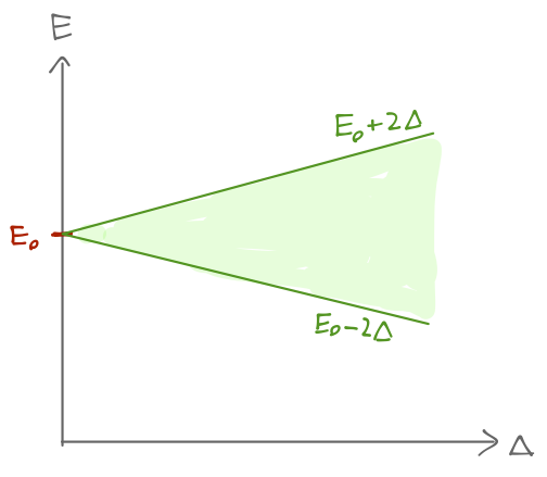
So as a result of the interaction term \( \Delta \), our single, discrete bound-state energy has split into a continuous band of energies in the range \( E \in [E_0 - 2\Delta, E_0 + 2\Delta] \).
The wavefunctions corresponding to these continuous energies should also look different, now that tunneling between wells is allowed. We know that for any particular choice of \( \theta \), the position-space wavefunction will be \( \sprod{x}{\theta} \). But now we notice that
\[ \begin{aligned} \bra{x} \hat{\tau}(a) \ket{\theta} = \sprod{x-a}{\theta} \\ = \sprod{x}{\theta} e^{-i\theta} \end{aligned} \]
letting \( \hat{\tau}(a) \) act to the left and then to the right. For these two quantities to be equal, the wavefunction must be (1) periodic under lattice translation, except for (2) a part which kicks out exactly \( e^{-i\theta} \) when we shift \( x \rightarrow x-a \). In other words, the wavefunction must take the form
\[ \begin{aligned} \sprod{x}{\theta} = e^{i\theta x/a} u_k(x), \end{aligned} \]
where \( u_k(x) \) is a periodic function with the same period as \( V(x) \), i.e. \( u_k(x+a) = u_k(x) \). The other piece here is a plane wave, from which we read off the wave number
\[ \begin{aligned} k = \theta/a. \end{aligned} \]
The observation above, that the wavefunction in the presence of a translation symmetry splits into a plane wave times a periodic function, is known as Bloch's theorem; the periodic functions themselves are called Bloch functions. Preferring to work with the wave number, we see that the physical states are now labelled by
\[ \begin{aligned} -\pi/a < k \leq \pi/a, \end{aligned} \]
and the corresponding bound-state energies are
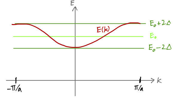
\[ \begin{aligned} E(k) = E_0 - 2\Delta \cos ka \end{aligned} \]
This range of allowed distinct values for \( k \) (or equivalently the range \( E_0 - 2 \Delta \leq E \leq E_0 + 2\Delta \)) is known as the Brillouin zone associated with this potential.
It's worth noting that the fact that we obtain a continuous band of energies \( E(k) \) is entirely because we have assumed that our potential is built from an infinite number of distinct, localized wells. We could have instead a finite chain of length \( N \), say with periodic boundary conditions so that translation from well \( N \) returns us back to well \( 1 \). Then we must have
\[ \begin{aligned} \bra{x} \hat{t}(a)^N \ket{\theta} = \sprod{x}{\theta} = \sprod{x-Na}{\theta} = \sprod{x}{\theta} e^{iN\theta} \end{aligned} \]
which gives us a quantization condition,
\[ \begin{aligned} \theta = \frac{2\pi}{N} j \end{aligned} \]
where \( j \) is an integer between \( (-N/2, N/2) \). So with a finite number of states to translate between, we return to the case of having a discrete number of energy levels.