Last time, we were studying periodic potentials and the physical implications of lattice translation symmetry. (One note in passing: in lecture, there was a bit of confusion about why the eigenvalues of the translation operator were pure phases \( e^{i\theta} \). I added a detailed discussion of this to the lecture notes from last time, but the short answer is "because the translation operator is unitary" - unitary operators have eigenvalues with unit norm.)
One general consequences of invariance under the lattice translation operator \( \hat{\tau}(a) \) was Bloch's theorem, that eigenfunctions of translation must take the form
\[ \begin{aligned} \sprod{x}{\theta} = e^{ik x} u_k(x), \end{aligned} \]
where \( k \equiv \theta/a \). When the state \( \ket{\theta} \) is also an energy eigenstate, the associated energy is given by the dispersion relation
\[ \begin{aligned} E(k) = E_0 - 2\Delta \cos ka. \end{aligned} \]
What does this equation really mean, and why is it called a "dispersion relation"? The short answer is that the relationship between energy and wave number is crucial in how quantum states evolve in time and space. Recall that for a plane wave solution, the time-dependent wavefunction is
\[ \begin{aligned} u_E(x,t) = Ae^{i(kx-\omega t)} + Be^{-i(kx+\omega t)} \end{aligned} \]
where \( \omega = E/\hbar \). A dispersion relation generalizes this form to systems where \( E(k) \) is different than the simple \( E \sim k^2 \) relationship for free particles. The exact form of the dispersion relation literally controls the dispersal of initial quantum states. (For example, a wave packet built of free plane waves will spread out in time. For a particle with linear dispersion, i.e. a photon \( \omega = ck \), then there is no dispersal; the shape of a wave packet would be fixed as time evolves.)
A detailed discussion of dispersion relations (and the related ideas of group/phase velocity) is somewhat useful, but not immediately useful for anything else we're going to do this semester. As a result I've decided to skip lecturing about dispersion relations in QM, but I will leave some bonus material in the lecture notes to read on your own - you're not expected to know this material.
Bonus material: Dispersion relations in quantum mechanics
(Full disclosure: for the below discussion, I am drawing heavily from Richard Fitzpatrick's online quantum notes.)
At this point, we have to go back and really dwell on the equation for \( E(k) \) above. This is an extremely important equation, with a name you'll hear frequently: the function \( E(k) \) is known as a dispersion relation, and it gives the relationship between energy and wave number. We've only seen one other example of a state with continuous energy values allowed, namely the plane wave; we can also write a disperion relation for plane waves, where \( k = \sqrt{2mE}/\hbar \):
\[ \begin{aligned} E(k) = \frac{\hbar^2 k^2}{2m} \end{aligned} \]
What does this equation actually mean, and why is it called a "dispersion relation"? To answer that, we need to go on a short digression back to time evolution and wave packets.
In most of our wave mechanics discussion so far, we've been dealing with plane wave solutions, e.g.
\[ \begin{aligned} u_E(x) = Ae^{ikx} + Be^{-ikx} \end{aligned} \]
These are the unique solutions to the (time-independent) Schrödinger equation in the presence of a constant potential. Of course, these are just solutions for the energy eigenfunctions associated with a particular \( E \); we add time-evolution back in by recalling that energy eigenstates evolve by picking up a pure phase:
\[ \begin{aligned} u_E(x,t) = Ae^{i(kx-\omega t)} + Be^{-i(kx+\omega t)} \end{aligned} \]
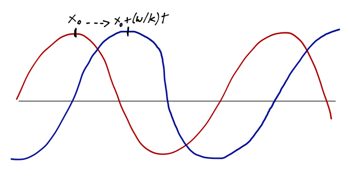
where \( \hbar \omega = E \). Each plane wave is represented as a pure phase, \( e^{i\phi} \). Moreover, we see that the value of the phase repeats in time, e.g. for wave \( A \):
\[ \begin{aligned} kx = k\left(x+\frac{\omega}{k} t \right) - \omega t \\ \Rightarrow \phi(x,0) = \phi(x+\frac{\omega}{k} t,t). \end{aligned} \]
We identify \( v_p \equiv \omega / k \) as the phase velocity associated with our (right-moving) plane wave, \( A \). Similarly, wave \( B \) moves to the left with the same phase velocity.
A plane wave clearly represents a moving particle, in some way. In fact, we have observed before that the plane wave \( e^{ikx} \) is in fact a momentum eigenstate, with eigenvalue \( p = \hbar k \) (and similarly, \( p=-\hbar k \) for the left-moving wave.) However, we notice something odd if we plug in the dispersion relation for a free particle to find the phase velocity:
\[ \begin{aligned} E(k) = \frac{\hbar^2 k^2}{2m} = \hbar \omega \\ \Rightarrow v_p = \frac{\omega}{k} = \frac{\hbar k}{2m} = \frac{p}{2m}. \end{aligned} \]
This is only half of the classical momentum of a single particle! Why is there a discrepancy?
We have to remember that a plane wave is something of an odd object. For simplicity I will set \( B=0 \) and focus on a right-moving plane wave. If we're going to try to do an experiment to find out the velocity of our particle, we have to measure its position at successive times: Born's rule tells us that the probability of any outcome is
\[ \begin{aligned} p(x) = \int_{-\infty}^\infty dx' \delta(x-x') |\psi(x',t)|^2 = |\psi(x,t)|^2. \end{aligned} \]
But for a plane wave, \( |\psi(x,t)|^2 \) is a constant, \( A^2 \)! So we're equally likely to find our particle anywhere, at any \( t \), regardless of the phase velocity. Thus we shouldn't be worried that the phase velocity doesn't equal the classical velocity, because the phase velocity clearly doesn't have the same physical meaning.
To make a proper comparison with the classical velocity of a particle, we have to start with a more localized state. I'll use a wave packet, which we've encountered before, but I should point out that we could choose a completely arbitrary initial wavefunction \( \psi(x,0) \). To find \( \psi(x,t) \), all we have to do is take the Fourier transform, which gives us the representation in terms of plane waves:
\[ \begin{aligned} \tilde{\psi}(k,0) = \frac{1}{\sqrt{2\pi}} \int_{-\infty}^\infty dx\ \psi(x,0) e^{-ikx} \end{aligned} \]
This relationship between momentum and position space holds at any \( t \) as well (the Fourier transform arises from the time-independent inner product \( \sprod{x}{p} \).) But now, since we are considering a free particle (the potential \( V(x) \) is constant), we can observe that \( [\hat{H}, \hat{p}] = 0 \), so the momentum eigenstates are also energy eigenstates. This means that the time-evolution in momentum space is very simple:
\[ \begin{aligned} \psi(k,t) = \sprod{k}{\psi(t)} = \bra{k} e^{i\hat{H} t/\hbar} \ket{\psi(0)} = e^{i\omega(k) t} \tilde{\psi}(k,0) \end{aligned} \]
where \( \omega(k) = E(k)/\hbar \). To go back to position space, we just Fourier transform again:
\[ \begin{aligned} \psi(x,t) = \frac{1}{\sqrt{2\pi}} \int_{-\infty}^\infty dk\ \tilde{\psi}(k,0) e^{i(kx-\omega(k) t)}. \end{aligned} \]
Note that these equations hold for any system in which the momentum is continuous and uniquely specifies the energy through a dispersion relation \( \omega(k) \), with some modification. (For the example of periodic structure that we saw above, the integral would just be over the Brillouin zone values of \( k \).)
Now let's specify the initial state to be a wave packet,
\[ \begin{aligned} \psi(x,0) \propto \exp \left( ik_0 x - \frac{(x-x_0)^2}{4(\Delta x)^2} \right) \end{aligned} \]
As we've seen before, this is a plane wave multiplied by a Gaussian "envelope"; the probability density \( |\psi(x,0)|^2 \) is pure Gaussian, centered at \( x_0 \) and with width \( (\Delta x) \). If we take the Fourier transform of a Gaussian, we find another Gaussian in momentum space:
\[ \begin{aligned} \tilde{\psi}(k,0) \propto \exp \left[ -ik x_0 - \frac{(k-k_0)^2}{4(\Delta k)^2} \right]. \end{aligned} \]
where \( \Delta k = 1 / (2 \Delta x) \); the wave packet saturates the uncertainty principle, as we've seen previously.
From above, the evolution of our wave packet in time (in position space) is thus
\[ \begin{aligned} \psi(x,t) = \frac{1}{\sqrt{2\pi}} \int_{-\infty}^\infty dk\ \exp \left[ -ikx_0 - \frac{(k-k_0)^2}{4(\Delta k)^2} \right] e^{i \phi(k)} \end{aligned} \]
where I've defined the phase \( \phi(k) = kx - \omega(k) t \). Since our wave packet is sharply peaked around \( k=k_0 \), let's try to do a Taylor expansion of the phase \( \phi(k) \) about the same point:
\[ \begin{aligned} \phi(k) \approx \phi_0 + \phi'_0 (k-k_0) + \frac{1}{2} \phi''_0 (k-k_0)^2 \end{aligned} \]
where
\[ \begin{aligned} \phi_0 = k_0 x - \omega_0 t \\ \phi'_0 = \left. \frac{d\phi}{dk} \right|_{k=k_0} = x - \frac{d\omega}{dk} t \\ \equiv x - v_g t \\ \phi''_0 = \left. \frac{d^2 \phi}{dk^2} \right|_{k=k_0} = -\frac{d^2 \omega}{dk^2} t \\ \equiv -\alpha t \end{aligned} \]
Plugging back in, we find
\[ \begin{aligned} \psi(x,t) \propto e^{i (k_0 x - \omega_0 t)} \int_{-\infty}^\infty dk\ \exp \left[ i(k-k_0) \left( x-x_0 - v_g t\right) - (k-k_0)^2 \left( \frac{1}{4(\Delta k)^2} + i \alpha t) \right) \right]. \end{aligned} \]
You'll recognize this as a Gaussian integral; with some appropriate changes of variables we can reduce the integrand to something of the form \( e{-u2} \) and then do it. I'll just tell you the result, up to overall constants:
\[ \begin{aligned} \psi(x,t) \propto \frac{1}{\sqrt{1+2\alpha i (\Delta k)^2 t}} \exp \left[ i(k_0 x - \omega_0 t) - (x-x_0 - v_g t)^2 \{ 1 - 2\alpha i (\Delta k)^2 t\} / (4\sigma(t)^2) \right]. \end{aligned} \]
with
\[ \begin{aligned} \sigma^2(t) = (\Delta x)^2 + \frac{\alpha^2 t^2}{4 (\Delta x)^2}. \end{aligned} \]
At \( t=0 \) this reduces to our original formula for the wave packet, which is a good cross-check. This formula is a little intimidating, but if we square it to find the probability density for finding our particle at position \( x \), it becomes illuminating:
\[ \begin{aligned} |\psi(x,t)|^2 \propto \frac{1}{\sigma(t)} \exp \left[ -\frac{(x-x_0 - v_g t)^2}{2 \sigma^2(t)} \right]. \end{aligned} \]
This is, once again, a Gaussian distribution, but with the peak translated from \( x_0 \) to \( x_0 + v_g t \). So the constant \( v_g = d\omega / dk \) is exactly what we should interpret as the analogue of the classical speed of our particle; it determines the rate at which the most likely outcome of measuring \( x \) changes. \( v_g \) is called the group velocity. It's easy to check that the dispersion relation for a free particle gives us
\[ \begin{aligned} v_g = \frac{p}{m}, \end{aligned} \]
matching on to the classical expectation. So to summarize, the center of a wave packet travels at the group velocity \( v_g = d\omega / dk \), while the phase of a plane wave changes with the phase velocity \( v_p = \omega / k \). The wave packet is the closest analogue to a classical experiment involving a single particle; a plane wave is better thought of as a continuous stream of particles moving in one direction.
One other observation we can make from our result for the evolution of a wave packet is that although it remains Gaussian, the width of the packet \( \sigma(t) \) increases over time, according to the constant \( \alpha = d^2 \omega / dk^2 \), which is commonly called the "group velocity dispersion" or sometimes just "the dispersion". Since \( \sigma(t) \sim \alpha^2 \), you can see that whatever the sign of \( \alpha \), the wave packet will spread out over time; the only exception is when \( \alpha = 0 \). This is the case for systems with linear dispersion relations, \( \omega(k) = ck \); light waves are one example. Linear dispersion also leads to the property that \( v_p = v_g \), i.e. light waves and light pulses travel at the same speed, \( c \).
Example: periodic delta functions
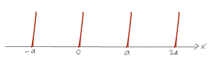
Let's go back to periodic symmetry and try an explicit example with a simple model: a periodic array of identical delta functions,
\[ \begin{aligned} V(x) = \sum_{n=-\infty}^\infty V_0 \delta(x-na) \end{aligned} \]
where I'm assuming \( V_0 > 0 \).
From our derivation before, we know that a general energy eigenstate can be written as a Bloch function times a plane wave,
\[ \begin{aligned} \psi(x) = e^{ikx} u_k(x) \end{aligned} \]
where \( u_k(x+a) = u_k(x) \). We also know that the full wavefunction between the delta functions must look like the sum of plane waves alone,
\[ \begin{aligned} \psi(x) = A e^{iqx} + B e^{-iqx}, \end{aligned} \]
where \( E(q) = \hbar^2 q^2 / (2m) \). Comparing the two equations, we see that the Bloch function has to be
\[ \begin{aligned} u_k(x) = A e^{i(q-k)x} + B e^{-i(q+k)x}. \end{aligned} \]
Now we apply the boundary conditions. Since \( u_k(0) = u_k(a) \), we see that
\[ \begin{aligned} A + B = A e^{i(q-k)a} + B e^{-i(q+k)a}. \end{aligned} \]
The other boundary condition, which you're now quite familiar with from the homework, is that the derivative \( \psi'(x) \) will have a specific discontinuity due to the delta functions:
\[ \begin{aligned} \psi'(\epsilon) - \psi'(-\epsilon) = \frac{2mV_0}{\hbar^2} \psi(0) = \frac{2mV_0}{\hbar^2} (A+B). \end{aligned} \]
Exploiting the periodicity of the wavefunction, we can write \( \psi'(-\epsilon) = \psi'(a-\epsilon) e^{-ika} \). Combining, we find the boundary condition
\[ \begin{aligned} \frac{2mV_0}{\hbar^2} (A+B) = iq[A (1-e^{i(q-k)a}) - B (1-e^{-i(q+k)a})]. \end{aligned} \]
Solving the two boundary conditions gives us a transcendental equation relating \( k \) and \( q \):
\[ \begin{aligned} \cos (ka) = \cos (qa) + \frac{mV_0}{\hbar^2} \frac{\sin(qa)}{qa}. \end{aligned} \]
Now we recall that \( q \) determines the energy of our state, \( E = \hbar^2 q^2 / 2m \). In the limit \( q \rightarrow \infty \), we just have \( \cos (ka) = \cos (qa) \), and we recover the standard free-particle dispersion \( E(k) = \hbar^2 k^2 / 2m \). However, for smaller values of \( qa \), the right-hand side of this equation can be larger than 1 (or smaller than -1), whereas the left-hand side can't be.
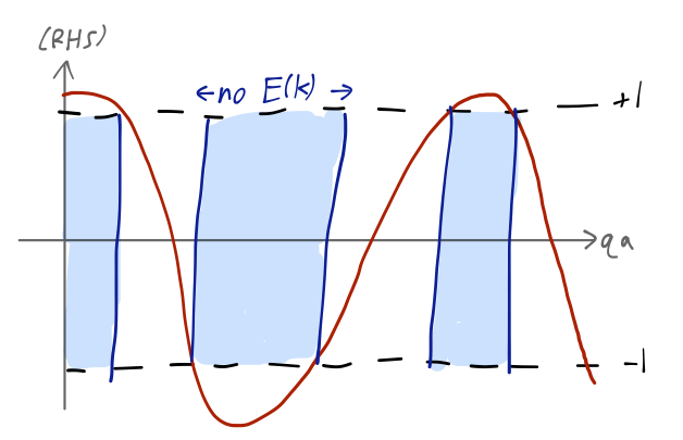
So certain values of \( E \) (and thus \( q \)) can never satisfy this equation. When the right-hand side of this equation is between -1 and 1, we find a continuum \( E(k) \) of possible energies, known as a band. The forbidden regions between the bands are known as band gaps.
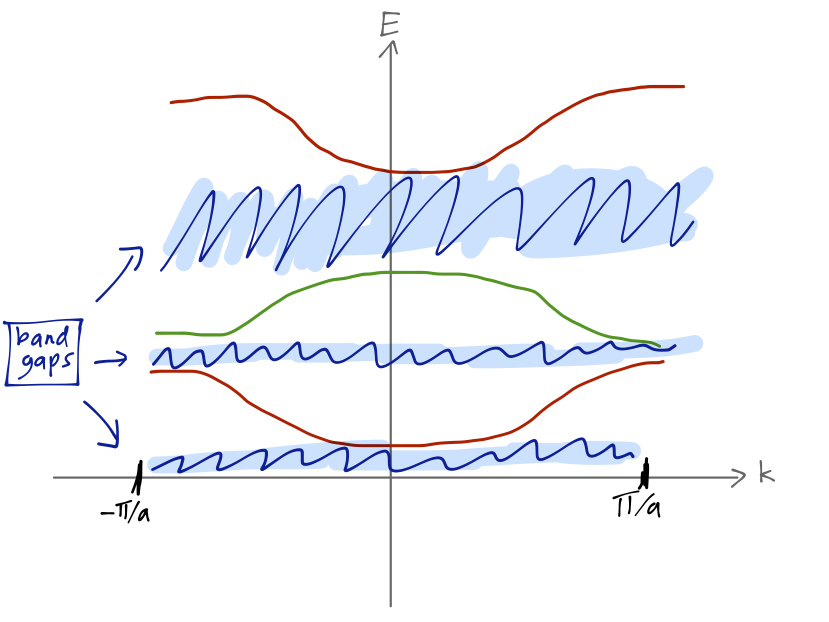
Some bands have much larger separations in energy than others. If you imagine the bands as being filled with single electrons, you can begin to see the difference between a metal (in which it's easy to excite an electron out of the ground state), and an insulator (in which it isn't easy.)
Continuous symmetries in quantum mechanics
We've seen now a few example of symmetries, i.e. operations under which a particular physical system is invariant. We've constructed explicit operators corresponding to these symmetries, and so far the operators have always been unitary. This is more than a coincidence; almost all symmetry operations in quantum mechanics correspond to unitary operators. The argument is straightforward:
- A symmetry can be considered as a transformation \( \hat{T} \) acting on the entire Hilbert space, i.e. all states are transformed from \( \ket{\psi} \rightarrow \hat{T} \ket{\psi} \).
- If \( \hat{T} \) is a symmetry of a particular Hilbert space, then all physical statements before and after applying \( \hat{T} \) must be the same.
- By Born's rule, the probability of observing outcome \( x \) from state \( \ket{\psi} \) is \( |\sprod{x}{\psi}|^2 \). This must be invariant under \( \hat{T} \), so we find
\[ \begin{aligned} |\bra{x} \hat{T}{}^\dagger \hat{T} \ket{\psi}|^2 = |\sprod{x}{\psi}|^2 \end{aligned} \]
for any \( x \) and any \( \ket{\psi} \).
This almost guarantees that a symmetry operator \( \hat{T} \) must be unitary. In fact, a result known as Wigner's theorem, which I won't attempt to prove here, guarantees that \( \hat{T} \) is either unitary or anti-unitary, the latter having the odd-looking property that \( \bra{x} \hat{T}^\dagger \hat{T} \ket{y} = \sprod{y}{x} \). Almost every symmetry in quantum mechanics is unitary, the most important anti-unitary example being the somewhat esoteric time-reversal symmetry. (I won't discuss time-reversal, but you can find a detailed treatment in Sakurai 4.4 if you're interested.)
It is a general fact that if we have a Hermitian operator \( \hat{Q} \), then we can construct a unitary operator by exponentiating it:
\[ \begin{aligned} \hat{U}(a) = \exp \left( -\frac{i \hat{Q} a}{\hbar} \right) \end{aligned} \]
(The sign and the presence of \( \hbar \) are by convention.) It should be clear that for Hermitian \( \hat{Q} \), we have \( \hat{U}^\dagger \hat{U} = 1 \). In fact, what we've constructed here is a whole family of unitary operators, parameterized by the arbitrary constant \( a \). We've seen an example of this construction before: the unitary time-translation operator, \( e^{-i\hat{H} t/\hbar} \).
What about the translation operator \( \hat{\tau}(L) \) which we just defined? We saw that for certain systems obeying "lattice translation symmetry", we only have invariance under translation for specific values of \( L \). However, there do exist systems (the isolated free particle being the simplest example) which are invariant under \( \hat{\tau}(L) \) for any choice of \( L \). In this case, we can study what happens when the translation becomes very small:
\[ \begin{aligned} \bra{x} \hat{\tau}(\epsilon) \ket{\psi} = \psi(x-\epsilon). \end{aligned} \]
We know that \( \epsilon = 0 \) corresponds to no translation at all, i.e. \( \hat{\tau}(0) = 1 \). Therefore, in the limit of small \( \epsilon \) we must be able to rewrite
\[ \begin{aligned} \hat{\tau}(\epsilon) = 1 - \frac{i\epsilon}{\hbar} \hat{G} + ... \end{aligned} \]
for some operator \( \hat{G} \). Expanding both sides of the above equation then gives us
\[ \begin{aligned} \sprod{x}{\psi} - \frac{i\epsilon}{\hbar} \bra{x} \hat{G} \ket{\psi} = \psi(x) - \epsilon \frac{d\psi}{dx}. \end{aligned} \]
So for spatial translations, \( \hat{G} \) is just the momentum operator, \( \hat{p} \). Although we've only shown that momentum gives rise to infinitesmal translations, we can "build up" a finite translation operator as a series of many infinitesmal ones:
\[ \begin{aligned} \hat{\tau}(a) = \lim_{N \rightarrow \infty} \left(1 - \frac{i \hat{p}}{\hbar} \frac{a}{N} \right)^N = \exp \left( -\frac{i \hat{p} a}{\hbar}\right). \end{aligned} \]
This ties back in to our discussion about exponentiated operators. Of course, we can always go the other way; if a symmetry operator is written as the exponential of a Hermitian operator \( \hat{Q} \), we can always expand for infinitesmal transformations:
\[ \begin{aligned} \hat{U}(\epsilon) = \exp \left( - \frac{i \hat{Q} \epsilon}{\hbar} \right) \rightarrow 1 - \frac{i}{\hbar} \hat{Q}\ \epsilon. \end{aligned} \]
We say that the Hermitian operator \( \hat{Q} \) inside the exponent is the generator of the corresponding symmetry. So the Hamiltonian is the generator of time translations, and the momentum operator is the generator of spatial translations.
These are all examples of continuous symmetries, since they depend on a continuous parameter. This is the alternative to a discrete symmetry, such as parity or lattice translation, where there is no "infinitesmal" version that we can build the full symmetry operator up from. As the name implies, discrete symmetries generally have a discrete (i.e. finite) set of eigenvalues and eigenvectors; parity has just two. Lattice translation on a ring of \( N \) atoms has \( N \) eigenvalues. (Lattice translation on an infinite chain is sort of an edge case; you can think of it as an infinite limit of a finite symmetry.)
For any symmetry, we may find that in addition to the states of our Hilbert space, some operators are left invariant as well, i.e.
\[ \begin{aligned} \bra{\psi} \hat{U}{}^\dagger \hat{A} \hat{U} \ket{\psi} = \bra{\psi} \hat{A} \ket{\psi}. \end{aligned} \]
Since \( \hat{U} \) is unitary, this is equivalent to the condition
\[ \begin{aligned} [\hat{A}, \hat{U}] = 0. \end{aligned} \]
Moreover, if \( \hat{U} \) is continuous, then we can write \( \hat{U} = 1 - i \hat{Q} (\Delta a) / \hbar + ... \), and so this immediately implies that
\[ \begin{aligned} [\hat{A}, \hat{Q}] = 0. \end{aligned} \]
For symmetries of the Hamiltonian, this has a particularly important consequence; we find that if \( [\hat{H}, \hat{U}] = 0 \) and \( \hat{U} \) is a continuous symmetry generated by \( \hat{Q} \), then \( [\hat{H}, \hat{Q}] = 0 \), and so
\[ \begin{aligned} [\hat{U}, \hat{H}] = 0 \Rightarrow \frac{d\hat{Q}}{dt} = 0. \end{aligned} \]
Thus we have the statement that for any continuous symmetry of the Hamiltonian, the corresponding generator is a conserved quantity. In classical mechanics, this familiar result is known as Noether's theorem; the quantum version is much simpler to derive, but no less powerful. So, from the examples we've seen, invariance of a physical system under translations in space and time lead to conservation of momentum and energy, respectively.
It is a fact that all known interactions do conserve energy and momentum; so as long as we take all of the interactions into account (so that we have no "external" sources or potentials), we will find that infinitesmal translation in time and space is always a symmetry. In other words, the position of an electron inside a crystal is not invariant except for discrete shifts by the lattice spacing \( x=a \); however, if we pick up the whole experiment, electron and crystal, and move it somewhere else in space, we expect that the outcomes will be identical.