Last time, we ended by discussing continuous symmetries: symmetry operations that include a continuous free parameter. The standard example is translation symmetry, which we studied last time, finding that translations are generated by the momentum operator, i.e. the translation operator can be written as
\[ \begin{aligned} \hat{\tau}(a) = \exp \left( -\frac{i\hat{p} a}{\hbar} \right). \end{aligned} \]
The correspondence between the unitary symmetry operator and a Hermitian generator of the symmetry is ubiquitous for continuous symmetries. In fact, it's more or less required if we insist that our continuous symmetry operator \( \hat{C}_a \) has three properties:
- Composition:
\[ \begin{aligned} \hat{C}_a \hat{C}_b = \hat{C}_{a+b} \end{aligned} \]
- Identity transformation:
\[ \begin{aligned} \hat{C}_0 = \hat{1} \end{aligned} \]
- Inverse + unitarity:
\[ \begin{aligned} \hat{C}_a^{-1} = \hat{C}_a^{\dagger} = \hat{C}_{-a}. \end{aligned} \]
The last two properties tell us immediately that for infinitesmal parameter value \( \epsilon \),
\[ \begin{aligned} \hat{C}_\epsilon = \hat{1} - i\epsilon \hat{G} / \hbar \end{aligned} \]
for Hermitian generator \( \hat{G} \), so that
\[ \begin{aligned} \hat{C}_\epsilon \hat{C}_{-\epsilon} = \hat{1} \end{aligned} \]
at first order in \( \epsilon \). We can then derive the exponential map for arbitrary \( a \), by repeatedly applying infinitesmal transformations or by using composition to derive a differential equation. (See Merzbacher 4.6.)
Basically, this is the observation that since we allow arbitrarily small continuous parameters we have a group structure which is smoothly connected to the identity. The more mathematical version of this statement is that these relations, and the exponential map from generator to unitary transformation, hold if the symmetry is a Lie group. As far as I know, all continuous symmetry groups in physics are Lie groups.
Obviously, symmetry is tremendously important in physics, and in fact most of the rest of this semester will be devoted to studying two other continuous symmetries: gauge symmetry, which is an important symmetry of electromagnetic fields that takes on new life in the quantum world, and rotational symmetry which will lead to angular momentum. We'll start with the shorter discussion, which will be gauge symmetry, but first we need to develop some new formalism.
Time evolution and propagators
We've seen a few specific examples of how to calculate time evolution in wave mechanics, particularly with the wave packet last time. The overall procedure is straightforward, but has several steps. First, if we can find some operator \( \hat{A} \) which commutes with the Hamiltonian, then we can construct a set of simultaneous eigenvectors, i.e. to each eigenvector \( \ket{a} \) of \( \hat{A} \) we can assign a unique energy \( E_a \). We can then calculate the time evolution of an arbitrary state by expanding in these eigenkets,
\[ \begin{aligned} \ket{\psi(t)} = \exp \left[ \frac{-i \hat{H} (t-t_0)}{\hbar} \right] \ket{\psi(t_0)} \\ = \sum_a \ket{a} \sprod{a}{\psi(t_0)} \exp \left[ \frac{-i E_a (t-t_0)}{\hbar} \right]. \end{aligned} \]
We can apply \( \bra{x} \) to both sides to see how the wavefunction in position space evolves:
\[ \begin{aligned} \sprod{\vec{x}}{\psi(t)} = \sum_a \sprod{\vec{x}}{a} \sprod{a}{\psi(t_0)} \exp \left[ \frac{-i E_a (t-t_0)}{\hbar} \right]. \end{aligned} \]
The second inner product here is exactly the expansion coefficients of the wavefunction for the \( \hat{A} \) eigenbasis: we can write
\[ \begin{aligned} \sprod{a}{\psi(t_0)} = \int d^3x' \sprod{a}{\vec{x}'} \sprod{\vec{x}'}{\psi(t_0)}. \end{aligned} \]
Combining these two expressions lets us rewrite the time-evolved wavefunction as an integral transformation from some initial time \( t_0 \), by inspection:
\[ \begin{aligned} \psi(\vec{x}',t) = \int d^3x K(\vec{x}',t; \vec{x}, t_0) \psi(\vec{x}, t_0) \end{aligned} \]
where the kernel function \( K \) is equal to
\[ \begin{aligned} K(\vec{x}', t; \vec{x}, t_0) = \sum_a \sprod{\vec{x}'}{a} \sprod{a}{\vec{x}} \exp \left[ \frac{-i E_a (t-t_0)}{\hbar} \right]. \end{aligned} \]
This kernel function \( K \) is called the propagator.
If you think back to our analysis of the time evolution of the wave packet, where we had to go through a complicated set of Fourier transforms, you can see the appeal of this approach; once we solve for the propagator for a particular operator \( \hat{A} \) which commutes with our Hamiltonian, then we can immediately write the time evolution of any wavefunction as an integral.
This form reinforces the point that quantum mechanics is perfectly causal; once we specify \( \psi(\vec{x}, t_0) \) and solve for the propagator, the wavefunction is totally determined for all time - as long as we don't disturb the system by making a measurement, which uncontrollably and abruptly changes the state into one of the eigenstates of that observable.
Notice that the propagator can be written compactly as the matrix elements of the time-evolution operator in coordinate space:
\[ \begin{aligned} K(\vec{x}', t; \vec{x}, t_0) = \sum_a \sprod{\vec{x}'}{a} \exp \left[ \frac{-i E_a (t-t_0)}{\hbar} \right] \sprod{a}{\vec{x}} \\ = \bra{\vec{x}'} \exp \left[ \frac{-i \hat{H} (t-t_0)}{\hbar} \right] \ket{\vec{x}}. \end{aligned} \]
In the limit \( t \rightarrow t_0 \), the operator in the middle approaches the identity and we have simply
\[ \begin{aligned} \lim_{t \rightarrow t_0} K(\vec{x}', t; \vec{x}, t_0) = \delta^3 (\vec{x}' -\vec{x}). \end{aligned} \]
Physically, we can interpret the propagator itself as a function of \( \vec{x}' \) and \( t \) as the time-evolved wavefunction of a particle localized exactly at position \( \vec{x} \) at initial time \( t_0 \). In fact, treating the propagator as a wavefunction itself, it's clear that it is a solution to the Schrödinger equation:
\[ \begin{aligned} \left[ - \frac{\hbar^2}{2m} (\nabla')^2 + V(\vec{x}') - i \hbar \frac{\partial}{\partial t} \right] K(\vec{x}', t; \vec{x}, t_0) = -i \hbar \delta^3 (\vec{x}' - \vec{x}) \delta(t-t_0), \end{aligned} \]
subject to the boundary condition \( K(\vec{x}', t; \vec{x}, t_0) = 0 \) for \( t < t_0 \), i.e. the solution is explicitly for times after \( t_0 \). (Those of you familiar with integral solutions to differential equations, especially in electrostatics, might recognize the propagator \( K \) as nothing more than the Green's function for the time-dependent Schrödinger equation.)
Let's go back to the case of the free particle in one dimension, \( \hat{H} = \hat{p}^2 / (2m) \). A good choice (really the only choice) for an observable commuting with \( \hat{H} \) is the momentum itself. This gives for the propagator
\[ \begin{aligned} K(x', t; x, t_0) = \bra{x'} e^{-i\hat{H} t/\hbar} \ket{x} \\ = \int dp \sprod{x'}{p} e^{-ip^2 t/2m\hbar} \sprod{p}{x} \\ = \frac{1}{2\pi \hbar} \int dp\ \exp \left[ \frac{ip (x'-x)}{\hbar} - \frac{ip^2 (t-t_0)}{2m\hbar} \right] \\ = \sqrt{\frac{m}{2\pi i \hbar (t-t_0)}} \exp \left[ \frac{im(x'-x)^2}{2\hbar (t-t_0)} \right] \Theta (t-t_0) \end{aligned} \]
where I've done the integral by completing the square to write it as a standard Gaussian, and I've added the Heaviside function to remind us that the propagator only applies for \( t > t_0 \). You can verify that if we set the initial state \( \psi(x,0) \) to be a wave packet, then using this propagator will allow us to recover the time-evolved form that we derived before. It's also possible to derive a closed-form expression for the propagator of the simple harmonic oscillator; I won't repeat the derivation here because it's not very enlightening, but you can find it in Sakurai.
Propagators can be joined together (or split apart) in a simple way; if we insert a complete set of position states into the definition of a single propagator, we see that
\[ \begin{aligned} K(x',t; x, t_0) = \int d^3 x'' \bra{x'} e^{-i \hat{H} (t - t')/\hbar} \ket{x''} \bra{x''} e^{-i \hat{H} (t'-t_0)/\hbar} \ket{x} \\ = \int d^3 x'' [K(x',t; x'', t') \times K(x'', t'; x, t_0)]. \end{aligned} \]
Aside from its practical application, there are some more general observations we can make from the propagator. Now I'll set \( t_0 = 0 \) for simplicity. If we set \( x' = x \) and integrate, we find a function only of time:
\[ \begin{aligned} G(t) \equiv \int d^3 x\ K(x, t; x, 0) \\ = \int d^3 x \sum_a \sprod{x}{a} \sprod{a}{x} e^{-iE_a t/\hbar} \\ = \sum_a \int d^3 x \sprod{a}{x} \sprod{x}{a} e^{-iE_a t/\hbar} \\ = \sum_a \sprod{a}{a} e^{-iE_a t/\hbar} \\ = \sum_a e^{-iE_a t/\hbar}. \end{aligned} \]
If you remember your statistical mechanics, you'll notice that this "sum over states" looks very similar to the partition function,
\[ \begin{aligned} Z = \sum_a e^{-\beta E_a} \end{aligned} \]
where \( \beta = 1/kT \). The analogue of \( \beta \) in our quantum equation is the quantity \( -it/\hbar \). As we will come to appreciate, there is significant overlap between the mathematics of propagators and that of statistical mechanics!
It's also interesting to consider a transformation of \( G(t) \) into a function of energy (this is an example of a Laplace transformation):
\[ \begin{aligned} \tilde{G}(E) \equiv -\frac{i}{\hbar} \int_0^\infty dt\ G(t) e^{iEt/\hbar} \\ = -\frac{i}{\hbar} \int_0^\infty dt\ \sum_a e^{-iE_a t/\hbar} e^{iEt/\hbar}. \end{aligned} \]
This is a purely oscillatory integral, but we can play a trick to get it to converge; if we allow the energy \( E \) to have an infinitesmal imaginary part, so \( E \rightarrow E + i \epsilon \), then the integral converges to
\[ \begin{aligned} \tilde{G}(E) = \sum_a \frac{1}{E - E_a + i\epsilon}. \end{aligned} \]
The function \( \tilde{G}(E) \) therefore encodes the entire energy spectrum of the theory; all of the distinct energy eigenvalues exist as poles in the complex plane. From our previous digression into complex energy, you can probably guess that this formula becomes important in the context of scattering states.
If we switch for a moment to the Heisenberg picture, there's another, possibly more intuitive way to represent exactly what the propagator is. Writing out the definition and doing some manipulations, we see that
\[ \begin{aligned} K(\vec{x}', t; \vec{x}, t_0) = \sum_a \sprod{\vec{x}'}{a} \sprod{a}{\vec{x}} \exp \left[ \frac{-i E_a (t-t_0)}{\hbar} \right] \\ = \sum_a \bra{\vec{x}'} \exp \left( -\frac{i\hat{H} t}{\hbar} \right) \ket{a} \bra{a} \exp \left( \frac{i \hat{H} t_0}{\hbar} \right) \ket{\vec{x}} \\ = \sprod{\vec{x}', t}{\vec{x}, t_0}. \end{aligned} \]
(You can tell we've switched to the Heisenberg picture because we're allowing the basis kets of \( \hat{x} \) to depend on time!) So the propagator is nothing more than the overlap of position ket \( \ket{\vec{x}} \) at time \( t_0 \) with a different position ket \( \ket{\vec{x}'} \) at later time \( t \). This overlap is known as the transition amplitude between these two states; taking the squared absolute value gives us the probability that, given we have observed the particle at \( \vec{x} \) at time \( t_0 \), we will find has transitioned to \( \vec{x}' \) at time \( t \).
Let's stick with Heisenberg picture for now, since it makes writing the propagator easier, and it also treats time and space a little more equally in the notation. It also makes certain properties seem much more obvious, like the composition property which we derived above, which just amounts to inserting a complete set of states:
\[ \begin{aligned} \sprod{\vec{x}', t'}{\vec{x}, t} = \int d^3 x'' \sprod{\vec{x}', t'}{\vec{x}'', t''} \sprod{\vec{x}'', t''}{\vec{x}, t}.\ \ (t < t'' < t') \end{aligned} \]
Note that there's no integral over time, just space; in the Heisenberg picture any operator commutes with itself at the same time, so we find the equal-time completeness relation
\[ \begin{aligned} \int d^3 x\ \ket{\vec{x}, t} \bra{\vec{x}, t} = 1. \end{aligned} \]
Time evolution can be tricky to think about in quantum mechanics, and the propagator formalism makes certain questions much easier to answer.
Example: the Moshinsky quantum race
An interesting application of the free-particle propagator is to a very simple experiment which sheds some light on the time evolution of particles in a quantum system, known as the Moshinsky quantum race. The idea is simple: we produce an (approximately) monochromatic beam of non-interacting particles, with some mass \( m \) and energy \( E \), which we can describe as a plane-wave state with wave number \( k = \sqrt{2mE}/\hbar \). The beam is sent into a barrier with a movable shutter in the center:
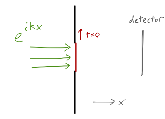
Until \( t=0 \), the shutter is closed and the wavefunction remains localized on the left side of the screen (\( x<0 \).) At \( t=0 \), we open the shutter; what does the profile of the traveling wave look like as time evolves? If we put a detection screen at some distance in front of the shutter, what will we observe?
The propagator makes these questions very straightforward to answer. The initial wavefunction is a plane wave trapped on the left side of the barrier, or
\[ \begin{aligned} \psi(x,0) = \Theta(-x) e^{ikx}. \end{aligned} \]
The wavefunction at time \( t \) is then just given by integrating this with the free propagator:
\[ \begin{aligned} \psi(x,t) = \int_{-\infty}^\infty dx' K_{\textrm{free}}(x,t; x',0) \psi(x',0) \\ = \sqrt{\frac{m}{2\pi i \hbar t}} \int_{-\infty}^0 dx' \exp \left[ \frac{i}{\hbar} \left( \frac{m (x-x')^2}{2t} + kx' \right) \right] \end{aligned} \]
I stopped here and left the integral for you; next time we'll look at the result.