Last time, I left you with an integral to do to find the wavefunction for the Moshinsky quantum race:
\[ \begin{aligned} \psi(x,t) = \sqrt{\frac{m}{2\pi i \hbar t}} \int_{-\infty}^0 dx' \exp \left[ \frac{i}{\hbar} \left( \frac{m (x-x')^2}{2t} + kx' \right) \right] \end{aligned} \]
Since we have an integral from \( -\infty \) to \( 0 \) and the function isn't even in \( x' \), this is a bit more complicated than just a Gaussian integral, but it's not too bad; Mathematica or some careful pen-and-paper work will give you the result
\[ \begin{aligned} \psi(x,t \geq 0) = \frac{1}{2} \exp \left( ikx - i k^2 \tau \right) {\rm erfc} \left( \frac{x-k\tau}{\sqrt{2i \tau}} \right) \end{aligned} \]
where \( \tau \equiv \hbar t/m \). "Erfc" is the complementary error function, equal to 1 minus the integral of a Gaussian curve; it looks like a smoother version of the Heaviside step function, equal to 1 at large, negative arguments and 0 for large and positive arguments. The total solution is a convolution of this shape with a plane wave, and looks something like this:
The wavefront here, defined as the point where the error function argument is zero, is at \( x = k \tau = \hbar k t / m = pt/m \), exactly how a classical particle would move. In the classical limit \( \hbar \rightarrow 0 \), the error function becomes infinitely steep, and we find a perfectly localized "wavefront", corresponding to the leading edge of the classical beam.
Quantum mechanically, this edge is smeared out; once we localized the wave at \( x=0, t=0 \), the evolution of different momentum components as a wave packet caused some spreading to occur. Still, if we performed the experiment of putting the screen in front of the shutter, we would find roughly zero probability of a particle hitting the screen for \( t < mx/\hbar k \), and roughly unit probability for \( t > mx/\hbar k \).
Example: the double-slit experiment
Another nice application of the free propagator is to one of the first experiments we encountered, which is the double-slit experiment:
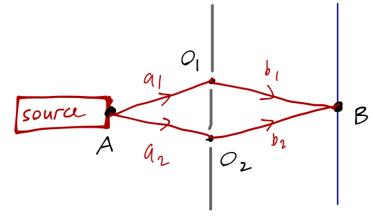
The wavefunction at point \( B \) on the screen at time \( t \) is given precisely by the propagator from the source at \( A \), \( \sprod{B, t}{A, 0} \). We can decompose this propagator into the product of propagators from \( A \) to the barrier, and from the barrier to \( B \). However, there are two possible paths now; the particle can either go through the upper opening \( O_1 \), or the lower opening \( O_2 \). From a probability point of view, these are completely independent events; the particle either goes through \( O_1 \) or \( O_2 \). Thus, the total probability amplitude can be written as a sum,
\[ \begin{aligned} \sprod{B,t}{A,0} = \int_0^t dt_1 \sprod{B,t}{O_1,t_1} \sprod{O_1,t_1}{A,0} + \int_0^t dt_2 \sprod{B,t}{O_2,t_2} \sprod{O_2,t_2}{A,0}. \end{aligned} \]
Each of the four individual propagators is nothing more than the free-particle propagator, for example
\[ \begin{aligned} \sprod{O_1,t_1}{A,0} = \left( \frac{m}{2\pi i \hbar t_1} \right) \exp \left( \frac{im a_1^2}{2\hbar t_1} \right) \end{aligned} \]
where I'm writing the propagator now in two dimensions, and \( a_1 \) is the distance from \( A \) to \( O_1 \). Thus, the product under the first integral becomes
\[ \begin{aligned} \sprod{B,t}{O_1,t_1} \sprod{O_1,t_1}{A,0} = \left( \frac{m^2}{4\pi^2 \hbar^2 t_1 (t-t_1)} \right) \exp \left[ \frac{im}{2\hbar} \left( \frac{a_1^2}{t_1} - \frac{b_1^2}{t-t_1} \right) \right] \end{aligned} \]
This is somewhat painful to integrate over, but if we plot the real part of the plane wave, we notice that as a function of the form \( e{ix2} \), it looks something like this:
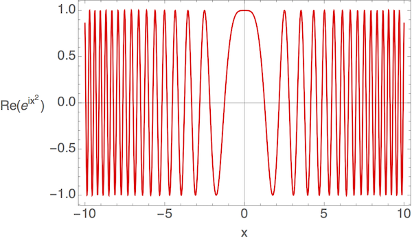
This function rapidly oscillates around zero if \( x \) is large, and so does the imaginary part. So we will find, on average, zero contribution to the integral from large values of \( x \). The integral should thus be dominated by the points where the argument of the exponential is near zero. Here, if we take \( a_1 \approx b_1 \), these points will be where \( t_1 \approx t-t_1 \). In fact, if we make the assumption that \( t_1 \approx t/2 \), we can rewrite the expression in the form
\[ \begin{aligned} \int_0^t dt_1 \sprod{B,t}{O_1,t_1} \sprod{O_1,t_1}{A,0} \approx \left( \frac{m^2}{\pi^2 \hbar^2 t^2} \right) \exp \left[ \frac{im}{\hbar t} (a_1 - b_1) (a_1 + b_1) \right] \end{aligned} \]
I leave it as an exercise to show that by taking approximations like the above in the appropriate way, for all four lengths \( a_i \) and \( b_i \) approximately equal (but not exactly equal) we find that the squared propagator takes on the familiar form of an interference pattern,
\[ \begin{aligned} |\sprod{B,t}{A,0}|^2 \propto 1 + \cos \left( \frac{m (\ell_1 - \ell_2) (\ell_1 + \ell_2)}{2\hbar t} \right) \sim \cos^2 \left( \frac{m (\ell_1 - \ell_2) (\ell_1 + \ell_2)}{4\hbar t} \right). \end{aligned} \]
where \( \ell_i = a_i + b_i \) is the total path length through each of the two slits.
Note: the \( 1/t \) may look funny, but remember that this is the propagator, which is only equal to the wavefunction if our initial state is really \( \ket{A,0} \), i.e. a sharp delta function localized at the source at time \( t=0 \). In this case, we expect non-trivial time dependence. If we have a steady-state source, we would remove \( t \) by identifying it as the time of flight from the source,
\[ \begin{aligned} t = \frac{\ell}{v} = \frac{m\ell}{p} = \frac{m\ell}{\hbar k} \end{aligned} \]
where \( \ell = (\ell_1 + \ell_2) / 2 \), so
\[ \begin{aligned} |\sprod{B,t}{A,0}|^2 \sim \cos^2 \left( \frac{k}{2} (\ell_1 - \ell_2) \right) = \cos^2 \left( \frac{\pi (\ell_1 - \ell_2)}{\lambda} \right), \end{aligned} \]
matching the textbook result based on wave interference.
We could at this point imagine generalizing this approach to deal with more complicated variants of the same problem. For example, if we had a barrier with three holes, or four, or \( N \) we could still find the final interference pattern just by summing over the possible propagator combinations:
\[ \begin{aligned} \sprod{B,t}{A_0} = \sum_{i=1}^N \int_0^t dt_i \sprod{B,t}{O_i,t_i}\sprod{O_i,t_i}{A,0}. \end{aligned} \]
A thought experiment: removing the screen
As this thought experiment becomes more complicated, it starts to lead us in an interesting direction. What if we added a second barrier in between the first and the detector?
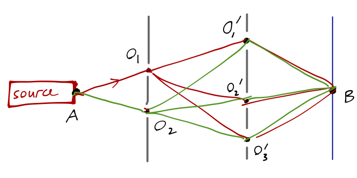
The events of the particle passing through any hole in any barrier are still all independent, so we can write the overall amplitude as a more complicated sum, decomposing into propagators from \( A \) to \( O_i \) to \( O'_j \) to \( B \). As we make this more and more complicated, with a greater number of barriers and a greater number of holes, the sum becomes more complicated, but the basic principle is still the same: we sum over the propagators for all possible paths that the particle can take from \( A \) to \( B \).
Now here is the important realization: if we take the limit where the number of holes in the barrier goes to infinity, so that there really isn't any barrier at all, then we're left with nothing but a particle propagating through empty space! But as we take the limit, we're still carefully summing over all of the number of possible paths, now approaching infinity. So screens or not, the probability ampltiude for a particle to propagate from \( x \) to \( y \) in time \( T \) is equal to the sum over all possible paths from \( x \) to \( y \). This was Richard Feynman's key insight into a new way of formulating quantum mechanics.
Let's go back to our rigorous definitions now. How do we formally describe such a "sum over paths"? Let's start by considering the interval from some initial time \( t_1 \) to final time \( t_N \), which we'll subdivide into \( N-1 \) equal steps in between:
\[ \begin{aligned} t_j - t_{j-1} = \frac{t_N - t_1}{N-1}. \end{aligned} \]
We'll also call the initial position \( x_1 \) and the final position \( x_N \). With no screens in the middle, we want to continuously average over the paths, so the sums become integrals:
\[ \begin{aligned} \sprod{x_N, t_N}{x_1, t_1} = \int dx_{N-1} \int dx_{N-2} ... \int dx_2 \\ \hspace{40mm} \sprod{x_N, t_N}{x_{N-1}, t_{N-1}} \sprod{x_{N-1}, t_{N-1}} ... \sprod{x_2, t_2}{x_1, t_1}. \end{aligned} \]
You'll immediately recognize this as just the application of the composition of propagators, as we defined above. In fact, we could have skipped the digression and just gone right to this equation, as Sakurai does. But I wanted to make the "sum over paths" idea a bit more clear. You should also suspect that this will be a particularly useful way to think about the case where \( \hat{H} \) depends explicitly on time (imagine a different \( \hat{H} \) appearing in each of the infinitesmal propagators.)
It's interesting to take another short digression and think about the classical version of this statement. Suppose we have the simple example of a particle moving subject to a gravitational force,
\[ \begin{aligned} \mathcal{L}_{\textrm{cl}} = \frac{1}{2} m \dot{z}^2 - mgz \end{aligned} \]
where the dot denotes a time derivative, \( \dot{z} = dz/dt \). We can similarly ask about the path from \( (z_1, t_1) \) to \( (z_N, t_N) \), and we're certainly free to subdivide the time interval in exactly the same way. But in classical mechanics, the motion is totally deterministic; once we specify the Lagrangian, \( z_1 \), and \( t_1 \), and the initial speed, the motion is completely determined, e.g. if we start at rest,
\[ \begin{aligned} (z_1, t_1) = (h, 0),\\ (z_2, t_2) = \left(h - \frac{1}{2} gt_2^2,t_2 \right)\\ \hspace{1mm} \\ ... \\ \hspace{1mm} \\ (z_N, t_N) = \left( 0 , \sqrt{\frac{2h}{g}} \right). \end{aligned} \]
As you know from classical mechanics, one way to derive this path is by considering multiple possible paths in the \( z-t \) plane: the unique classical path is the one which extremizes the action, \( S_{\textrm{cl}} = \int_{t_1}^{tN} \mathcal{L}{\textrm{cl}}(z, \dot{z}) \), leading to the Euler-Lagrange equations of motion.
The path integral
Now we're ready to return to the quantum expression for the propagator. Notice that we can rewrite each of the intermediate propagators by pulling out the time evolution to find
\[ \begin{aligned} \sprod{x_j, t_j}{x_{j-1}, t_{j-1}} = \bra{x_j} \exp \left( - \frac{i\hat{H} \Delta t}{\hbar} \right) \ket{x_{j-1}}. \end{aligned} \]
Since we're studying the evolution of a single particle, let's split the Hamiltonian up into the kinetic and potential energy terms,
\[ \begin{aligned} \hat{H} = \frac{\hat{p}^2}{2m} + V(\hat{x}). \end{aligned} \]
Since \( \hat{x} \) and \( \hat{p} \) don't commute, normally we wouldn't be able to split up the exponential. But since we're dealing with the infinitesmal time-step \( \Delta t \), we can rewrite
\[ \begin{aligned} \exp \left( -\frac{i\hat{H} \Delta t}{\hbar} \right) = \exp \left( -\frac{i \hat{p}^2 \Delta t}{2m \hbar} \right) \exp \left( -\frac{i V(\hat{x}) \Delta t}{\hbar} \right) + \mathcal{O}(\Delta t^2). \end{aligned} \]
Inserting a complete set of states then gives
\[ \begin{aligned} \sprod{x_j, t_j}{x_{j-1}, t_{j-1}} = \int dx' \bra{x_j} \exp \left( -\frac{i \hat{p}^2 \Delta t}{2m\hbar} \right) \ket{x'} \bra{x'} \exp \left( -\frac{i V(\hat{x}) \Delta t}{\hbar} \right) \ket{x_{j-1}} \\ = \int dx' \bra{x_j} \exp \left( -\frac{i \hat{p}^2 \Delta t}{2m\hbar} \right) \ket{x'} \exp \left( -\frac{i V(x_{j-1}) \Delta t}{\hbar} \right) \delta(x' - x_{j-1}). \end{aligned} \]
The first expression is just the free-particle propagator which we're now familiar with, and the delta function from the second term collapses the integral, so we have
\[ \begin{aligned} \sprod{x_j, t_j}{x_{j-1}, t_{j-1}} = \sqrt{\frac{m}{2\pi i \hbar \Delta t}} \exp \left[ \left( \frac{m(x_j - x_{j-1})^2}{2 (\Delta t)^2} - V(x_{j-1}) \right) \frac{i \Delta t}{\hbar} \right]. \end{aligned} \]
Plugging back in to the full propagator above, we thus find
\[ \begin{aligned} \sprod{x_N, t_N}{x_1, t_1} = \left( \frac{m}{2\pi i \hbar \Delta t}\right)^{(N-1)/2} \int dx_{N-1} dx_{N-2} ... dx_2 \\ \exp \left[ \frac{i \Delta t}{\hbar} \sum_{j=2}^{N-2} \left(\frac{1}{2} m \left( \frac{x_{j+1} - x_j}{\Delta t}\right)^2 - V(x_j) \right) \right] \end{aligned} \]
Finally taking the limit \( \Delta t \rightarrow 0 \), the difference becomes a derivative and the sum an integral:
\[ \begin{aligned} \lim_{\Delta t \rightarrow 0} \sprod{x_N, t_N}{x_1, t_1} = \int \mathcal{D}[x(t)] \exp \left[ \frac{i}{\hbar} \int_{t_1}^{t_N} dt \left( \frac{1}{2} m \dot{x}(t)^2 - V(x(t)) \right) \right]. \\ = \int_{x_1}^{x_N} \mathcal{D}[x(t)] \exp \left[ \frac{i}{\hbar} \int_{t_1}^{t_N} dt\ \mathcal{L}(x, \dot{x}) \right] = \int_{x_1}^{x_N} \mathcal{D}[x(t)] \exp \left[ \frac{iS(x,\dot{x})}{\hbar} \right]. \end{aligned} \]
This is the Feynman path integral. The script D denotes the "path integration" itself, which is the properly-normalized infinite-dimensional limit of our interval subdivision,
\[ \begin{aligned} \int_{x_1}^{x_N} \mathcal{D}[x(t)] \equiv \lim_{N \rightarrow \infty} \left( \frac{m}{2\pi i \hbar \Delta t} \right)^{(N-1)/2} \int dx_{N-1} \int dx_{N-2} ... \int dx_2. \end{aligned} \]
The quantity \( S = \int dt\ \mathcal{L} \) is the action, the same function which appears mysteriously in the derivation of the Lagrangian framework.
The path integral provides us with a very intuitive way of seeing how classical mechanics arises from quantum mechanics, and in particular why a classical system should satisfy the principle of least action. Suppose we want to compare the contribution of two paths to the overall propagator, one with action \( S_0 \), and another with action \( S_0 + \delta S \). As we've seen, the total contribution is the sum over the paths of \( e^{iS/\hbar} \), i.e.
\[ \begin{aligned} \exp \frac{i S_0}{\hbar} + \exp \left(\frac{i (S_0 + \delta S)}{\hbar} \right) = e^{iS_0 / \hbar} \left(1 + e^{i \delta S / \hbar} \right). \end{aligned} \]
If we average over many paths, "integrating" over \( \delta S \) in the formal sense, we see that if the changes in action are large compared to \( \hbar \), then the phase will oscillate wildly; as the phase varies, it will go from \( 1 \) to \( -1 \) and anywhere in between in the complex plane, and we can find large cancellations. The only sets of paths which will contribute significantly, similar to what we saw in the two-slit example above, are those which add coherently, i.e. for which \( \delta S \approx 0 \). Turning points of the action, where \( \delta S \) changes slowly as the path is deformed, are exactly those paths given by the Euler-Lagrange equations; they are the classical paths.