Last time, we ended by pushing the propagator formalism to its limit in deriving the Feynman path integral:
\[ \begin{aligned} \sprod{x_N, t_N}{x_1, t_1} = \int_{x_1}^{x_N} \mathcal{D}[x(t)] \exp \left[ \frac{i}{\hbar} \int_{t_1}^{t_N} dt\ \mathcal{L}(x, \dot{x}) \right] \end{aligned} \]
This gives a very different formulation of quantum mechanics, but one which is equivalent to the Schrödinger approach. we've been working in. In fact, it's possible (as you'll show on the homework) to start with the path integral and derive the time-dependent Schrödinger equation.
We can even solve for the dynamics of quantum systems using the path integral, at least in principle. As Sakurai points out, the path integral can be exactly evaluated for the simple harmonic oscillator, giving the propagator (and with a little more work, the energy eigenfunctions and corresponding energy levels.) Unfortunately, the path integral is intractable for all but the simplest non-relativistic quantum systems. Our goal will mostly be to use it as a formal construct, to give us useful insights into gauge symmetry that are much more obscure without the path integral.
In quantum field theory and statistical mechanics, the path integral sees much more practical use. In fact, there is a subfield known as lattice field theory which turns the infinite-dimensional path integral into a finite-dimensional object by discretizing space and time into a finite lattice, and then uses Monte Carlo methods to evaluate the path integral numerically. But that's a story for another class!
Potential energy and gauge transformation
We're now equipped to deal with a more subtle kind of symmetry, known as gauge symmetry. A gauge transformation, generally, can be thought of as a redefinition of the potential energy. The simplest example is a change of the form
\[ \begin{aligned} \tilde{V}(\vec{x}) = V(\vec{x}) + V_0, \end{aligned} \]
where \( V_0 \) is constant in both space and time. You can think of this as simply a redefinition of what we call the zero-point of energy, hence the name "gauge transformation" (we would have to relabel the "gauge" we use to measure \( V(x) \).)
Classically, adding a constant to our definition of potential has no effect at all on the physics; in terms of Newton's laws, the force depends only on the gradient of the potential, so we can add any constant we want.
Is the same statement true in quantum mechanics? We might be worried that it won't be, since if we look at the time-independent Schrödinger equation, we notice that the potential appears directly, without any derivative:
\[ \begin{aligned} -\frac{\hbar^2}{2m} \nabla^2 \psi + (V(\vec{x}) - E) \psi(\vec{x}) = 0. \end{aligned} \]
In fact, changing from \( V \) to \( \tilde{V} \) will affect the time evolution of our kets: we see that from some initial ket \( \ket{\alpha} \), we will find with the new potential
\[ \begin{aligned} \tilde{\ket{\alpha, t}} = \exp \left[ -i \left( \frac{\vec{p}^2}{2m} + V(\vec{x}) + V_0\right) \frac{t}{\hbar} \right] \ket{\alpha} \\ = e^{-iV_0 t/\hbar} \ket{\alpha, t}. \end{aligned} \]
So changing the zero of the potential changes our definition of the time-evolved ket by a phase. If \( \alpha \) is an energy eigenstate, then
\[ \begin{aligned} e^{-iV_0 t/\hbar} \ket{\alpha,t} = \exp \left( \frac{-i(E+V_0)t}{\hbar} \right) \ket{\alpha}. \end{aligned} \]
Thus, all we've done is replaced \( E \rightarrow E + V_0 \), as we should expect. In fact, nothing we can actually observe has changed; rescaling every ket in the Hilbert space by the same phase leaves all inner products and expectation values unchanged (as we've observed before.)
Although we have seen that a completely global rescaling of the potential energy has no physical effect, there are some rather large surprises lurking in the effects of local potential changes in quantum mechanics. As a first taste of this subject, consider an experiment involving two metallic cages, which are maintained at a constant potential difference. We take a beam of electrons and split it into two parts to pass through the two cages:
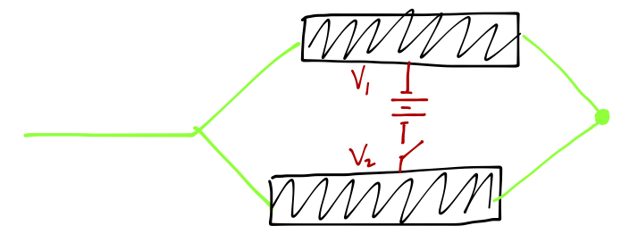
We switch the potential difference on only while the electrons are in the cages, so they never feel an electric force outside the cages. Within each cage, the electric potential is uniform, and so the particles again feel no force. However, there is a phase shift induced by the background potential, and the phase shift is different in each cage. Thus, if we recombine the beams at the other end of the cages, we find that the measured intensity of the recombined beam exhibits interference, with the intensity modulating according to the difference in phase shifts,
\[ \begin{aligned} I \sim \cos \left( \frac{1}{\hbar} \int dt\ [V_2(t) - V_1(t)] \right) \end{aligned} \]
You'll notice from the presence of \( \hbar \) that this is a purely quantum mechanical effect, which vanishes as \( \hbar \rightarrow 0 \) and the oscillations become infinitely fast. This is a first example of something which we will see in detail: although only the electromagnetic fields are "real" in classical theory, in quantum theory the electromagnetic potential fields themselves are more fundamental.
A slightly more elaborate but much more interesting example is given by an experiment known as the gravity interferometer. Rather famously, the unification of gravity and quantum mechanics is an unsolved problem to this day, but there are still quantum-mechanical effects that can be observed and explained perfectly in the presence of a background, classical gravitational field.
In classical mechanics, gravity is usually the first force which is encountered, partly because it is so simple to deal with: the classical equation of motion for a particle in the Earth's gravitational field is simply
\[ \begin{aligned} \vec{F} = m\ddot{z} = -mg \end{aligned} \]
and the mass cancels out, leaving a constant acceleration. What about the quantum system? Again for a particle moving in one dimension, we have
\[ \begin{aligned} \left[ - \left( \frac{\hbar^2}{2m}\right) \frac{d^2}{dz^2} + m\Phi_g \right] \psi(z) = i\hbar \frac{\partial \psi}{\partial t}. \end{aligned} \]
where \( \Phi_g = gz \) is the (approximate) gravitational potential field near the Earth's surface. Now the mass doesn't cancel; the best we can do is divide through, so that our equation depends only on the ratio \( \hbar/m \). Although the gravitational action is the same, the way it is treated in classical versus quantum physics leads to this difference: in the quantum system, the action appears in the path integral
\[ \begin{aligned} \sprod{z_f, t_f}{z_i, t_i} = \int \mathcal{D}[z(t)] \exp \left[ i \int_{t_i}^{t_f} dt \frac{1}{\hbar} \left( \frac{1}{2} m\dot{z}^2 - mgz \right) \right] \end{aligned} \]
which again depends on \( \hbar/m \), and in particular we can't factor out the mass in any way. On the other hand, for the classical action we're only interested in the stationary point
\[ \begin{aligned} \delta \int_{t_i}^{t_f} dt \left( \frac{1}{2} m\dot{z}^2 - mgz \right) = 0 \end{aligned} \]
and we can just divide both sides by \( m \) before we do the variation.
Of course, to first order the behavior of a quantum particle in a classical gravity field will just be free-fall, i.e. \( \frac{d^2 \ev{z}}{dt^2} = -g \). (This can be derived from the Schrödinger equation.) What we need to really see is a quantum effect, i.e. some dependence on \( \hbar/m \). Unfortunately, gravity is by far the weakest force. Sakurai points to the example of a hydrogen atom, in which an electron and proton are bound by the electromagnetic force; the approximate size of the atom is given by the Bohr radius,
\[ \begin{aligned} a_0 = \frac{\hbar^2}{e^2 m_e} \approx 0.025\ {\rm nm} \end{aligned} \]
If we tried to construct a similar "atom" from a neutron and electron, bound only by the gravitational force, the equivalent "Bohr radius" would be
\[ \begin{aligned} a_{0,g} = \frac{\hbar^2}{G_N m_e^2 m_n} \sim 10^{13}\ {\rm ly} \end{aligned} \]
which is (substantially) larger than the size of the entire universe!
So gravity is weak, but we can still observe its quantum effects if we come up with the right experiment. As I mentioned, a gravitational interferometer is the best example. Like the electric field example above, we prepare a beam of neutrons and split it along two different paths, \( A \to B \to D \) and \( A \to C \to D \):
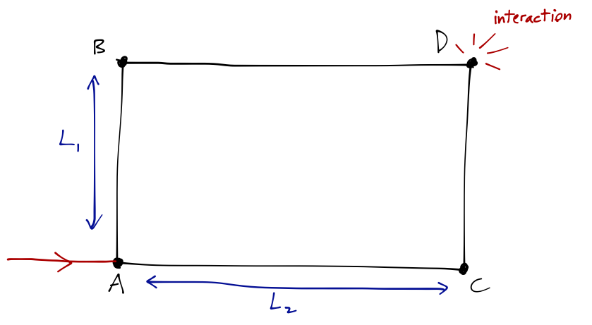
We imagine that the experiment is mounted on an adjustable platform, so that we can change the angle of gravity relative to the paths. If the plane of the paths is perfectly horizontal, then there is no effect, since the gravitational potential is constant everywhere. However, if we tilt to an angle \( \delta \) along the axis parallel to \( AC \), then path \( BD \) is at a higher potential than \( AC \) by an amount
\[ \begin{aligned} \Delta V = m_n g L_2 \sin \delta. \end{aligned} \]
The potential changes in the same way for traversing paths \( AB \) and \( CD \), so only the above potential difference is significant, and it leads to a phase shift at the interference point of
\[ \begin{aligned} \Delta \phi = \exp \left[ \frac{-i m_n g L_2 (\sin \delta) T}{\hbar} \right] \end{aligned} \]
where \( T \) is the time-of-flight. This is now an \( \hbar/m \) effect, and the dimensions actually work out nicely for a tabletop experiment; this formula was confirmed by just such an experiment in 1975, which you can see in Sakurai. Notice that just like the electron beam experiment, we are sensitive in quantum mechanics directly to the potential \( \Phi_g \) through the height difference \( (\sim \sin \delta) \), even though the gravitational acceleration itself is perfectly uniform even when we tilt the experiment.
One other aside before we keep moving: one of the reasons that we can cancel out the mass dependence in classical mechanics is the equivalence principle, i.e. the equality of inertial mass (the one that appears in \( F=ma \)) and gravitational mass. The \( m_n \) in the above formula is the gravitational mass, but the time-of-flight \( T \) depends on the inertial mass of the neutron, so we can think of the gravitational interferometer experiment as a test of the EP for a quantum-mechanical system.
The electromagnetic potential
As you know, potentials don't just appear as simple functions \( V(x) \); the electric and magnetic fields depend on both a scalar potential \( \phi \), and a vector potential \( \vec{A} \). Once again, we know that the (time-independent) classical EM fields are invariant under certain redefinitions of these potentials, in particular
\[ \begin{aligned} \phi \rightarrow \phi + \lambda \\ \vec{A} \rightarrow \vec{A} + \nabla \Lambda \end{aligned} \]
where \( \lambda \) and \( \Lambda \) may both be functions of position. Once again, we will find that the potential functions themselves are important in the quantum theory.
Let's start from the classical Hamiltonian for a charged particle in an electromagnetic field:
\[ \begin{aligned} H = \frac{1}{2m} \left( \vec{p} - \frac{e}{c} \vec{A}(\vec{x}) \right)^2 + e\phi(\vec{x}). \end{aligned} \]
This is simply a function of position and momentum, so to obtain the quantum Hamiltonian we just replace \( p \) and \( x \) with their operator counterparts. This is easier said than done, because now we have an ambiguity: there are multiple possible definitions of \( (p - eA/c)^2 \) involving products of \( \hat{\vec{p}} \) and \( \hat{\vec{A}} \) in different orders. We should certainly choose a Hermitian combination: let's take the choice
\[ \begin{aligned} \hat{\vec{p}}{}^2 + \frac{e^2}{c^2} \hat{\vec{A}}{}^2 - \frac{e}{c} \left( \hat{\vec{p}} \cdot \hat{\vec{A}} + \hat{\vec{A}} \cdot \hat{\vec{p}} \right). \end{aligned} \]
We'll start in the Heisenberg picture. Our first speed bump occurs in the time evolution of the \( \hat{\vec{x}} \) operator: for each component \( x_i \) we find
\[ \begin{aligned} \frac{d\hat{x}_i}{dt} = \frac{1}{i\hbar} [\hat{x}_i, \hat{H}] = \frac{1}{m} (\hat{p}_i - e\hat{A}_i/c). \end{aligned} \]
So \( m d\hat{x}_i / dt \neq \hat{p}_i \)! We define this new combination to be the kinematical momentum,
\[ \begin{aligned} \hat{\vec{\Pi}} = m \frac{d\hat{\vec{x}}}{dt} = \hat{\vec{p}} - \frac{e}{c} \hat{\vec{A}}. \end{aligned} \]
The original operator \( \hat{\vec{p}} \) is then called the canonical momentum; it's still the same \( \hat{\vec{p}} \) operator we're familiar with, and in particular it still satisfies the canonical commutation relations with \( \hat{\vec{x}} \). Unlike the canonical momentum, the different vector components of \( \hat{\vec{\Pi}} \) don't commute with each other: it's easy to verify that
\[ \begin{aligned} [\hat{\Pi}_i, \hat{\Pi}_j] = \left( \frac{i\hbar e}{c} \right) \epsilon_{ijk} \hat{B}_k, \end{aligned} \]
where \( \hat{B}_k \) is the magnetic field, \( \nabla \times \hat{\vec{A}} \). We can use this to derive the quantum version of the Lorentz force law:
\[ \begin{aligned} m \frac{d^2 \hat{\vec{x}}}{dt^2} = \frac{d\hat{\vec{\Pi}}}{dt} = e \left[ \hat{\vec{E}} + \frac{1}{2c} \left( \frac{d\hat{\vec{x}}}{dt} \times \hat{\vec{B}} - \hat{\vec{B}} \times \frac{d \hat{\vec{x}}}{dt} \right) \right]. \end{aligned} \]
As a brief aside, one of the other equations that changes is the continuity equation,
\[ \begin{aligned} \frac{\partial \rho}{\partial t} + \nabla \cdot \vec{j} = 0, \end{aligned} \]
which expresses probability conservation. For the electromagnetic Hamiltonian we still have \( \rho = |\psi|^2 \), but a careful re-derivation (look in Sakurai) reveals that the probability current is now
\[ \begin{aligned} \vec{j} = \frac{\hbar}{m} {\rm Im} (\psi^\star \nabla \psi) - \frac{e}{mc} \vec{A}(\vec{x}) |\psi|^2. \end{aligned} \]
You might feel uneasy that the vector potential itself appears directly in this equation; this is a much more tangible effect than the rescaling of the potential we saw before! In fact, the whole redefinition of the momentum operator in terms of \( \vec{A} \) looks very weird. On the other hand, the probability current is still sort of abstract; we should look for a real physical effect to untangle what is happening here.