Let me start by recapping quickly one important point from last time: our study of local gauge invariance started with the example of a gauge transformation of the electromagnetic potential of the form
\[ \begin{aligned} \phi \rightarrow \phi,\\ \vec{A} \rightarrow \vec{A} + \nabla \Lambda(\vec{x}), \end{aligned} \]
and argued that this leads to a transformation of the wavefunction by a phase which varies in space,
\[ \begin{aligned} \psi(x,t) \rightarrow \psi'(x,t) = e^{i \theta(x)} \psi(x,t). \end{aligned} \]
As was pointed out in class, it's not especially obvious that this transformation follows from the gauge transformation - although it is true. However, it's at least obvious that invariance under the local gauge transformation above will do something which is spatially dependent to the wavefunction, which motivated our study of what happens under the second equation.
The far more important observation is that if we start with the second equation and call that "gauge symmetry", then we can derive the transformation laws for the vector potential, and in fact the precise form of the electromagnetic interactions in quantum mechanics. For this reason, the second equation is generally taken to define a local gauge symmetry, and electromagnetism is identified as a gauge interaction.
The Aharonov-Bohm effect
Let's turn to another famous experimental result, which is often cited as further evidence for the "reality" of the gauge potential \( \vec{A} \) in quantum mechanics: the Aharonov-Bohm experiment.
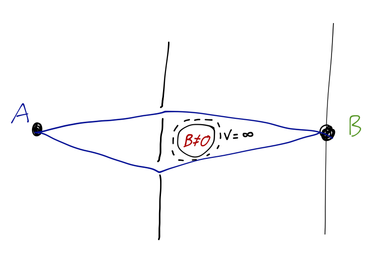
The original version of the Aharonov-Bohm effect, which is best understood using the path integral, is a straightforward modification of the double-slit experiment: along the path traveled by the particles, we add an impenetrable cylinder, containing a solenoid with uniform \( B \neq 0 \) perpendicular to the plane of the page.
Let's see what happens. Following our previous notation, we'll take \( \vec{x}_1 \) to be a point at the source \( S \), and \( \vec{x}_N \) to be a point somewhere in the interference or detection region, \( I \). To apply path integration, we need the classical Lagrangian to start with; similar to the Hamiltonian, it is derived by insisting that the classical equations of motion give us the Lorentz force law back. With the scalar potential set to zero, this leads to the result
\[ \begin{aligned} \mathcal{L} = \frac{1}{2} m \dot{\vec{x}}^2 + \frac{e}{c} \dot{\vec{x}} \cdot \vec{A}. \end{aligned} \]
We're mainly interested in the change in the action induced by this second term, when the vector potential is switched on. Along a particular path segment from \( (\vec{x}{n-1}, t{n-1}) \) to \( (\vec{x}_n, t_n) \), we have
\[ \begin{aligned} S = \int_{t_{n-1}}^{t_n} dt\ \mathcal{L} = S_0 + \int_{t_{n-1}}^{t_n} dt\ \frac{e}{c} \dot{\vec{x}} \cdot \vec{A} \\ = S_0 + \frac{e}{c} \int_{\vec{x}_{n-1}}^{\vec{x}_n} \vec{A} \cdot \vec{ds}. \end{aligned} \]
Thus, if we combine all of the infinitesmal paths together along our particle's trajectory, we just end up with the sum of all of these infinitesmal line integrals, which is equal to the total line integral over the path:
\[ \begin{aligned} e^{iS/\hbar} = e^{iS_0 / \hbar} \exp \left[ \frac{ie}{\hbar c} \int_{\vec{x}_1}^{\vec{x}_N} \vec{A} \cdot \vec{ds} \right]. \end{aligned} \]
This expression gives us the phase shift for one particular path, so now we have to carry out the sum over all possible paths. Fortunately, this is easier than it seems. As we just recalled above, the line integral of \( \vec{A} \) around any closed path is equal to the magnetic flux contained inside,
\[ \begin{aligned} \oint \vec{A} \cdot \vec{ds} = \Phi_{B, \textrm{int}}. \end{aligned} \]
Of course, if we take any path from \( S \) to \( I \), and combine it with a path back from \( I \) to \( S \), we have a closed path. Thus, if we combine two paths which both pass above or below the solenoid, the enclosed flux is zero, and we find
\[ \begin{aligned} \left[\int_S^I \vec{A} \cdot \vec{ds} + \int_I^S \vec{A} \cdot \vec{ds'}\right]_{\textrm{above}} = \left[\int_S^I \vec{A} \cdot \vec{ds} + \int_I^S \vec{A} \cdot \vec{ds'}\right]_{\textrm{below}} = 0 \end{aligned} \]
However, if we take one path above and one below, then the impenetrable cylinder is enclosed, and we have a non-zero difference,
\[ \begin{aligned} \left[ \left( \frac{e}{\hbar c}\right) \int_{\vec{x}_1}^{\vec{x}_N} \vec{A} \cdot \vec{ds} \right]_{\textrm{above}} - \left[ \left( \frac{e}{\hbar c}\right) \int_{\vec{x}_1}^{\vec{x}_N} \vec{A} \cdot \vec{ds} \right]_{\textrm{below}} = \frac{e \Phi_B}{\hbar c}. \end{aligned} \]
The contribution to the probability of observation at point \( \vec{x}_N \) (and thus the beam intensity) goes as the modulus squared of the amplitude, i.e. for two paths \( P_1 \) and \( P_2 \) we have
\[ \begin{aligned} I \supset \left| \int [dx]_{P_1} e^{iS/\hbar} \right|^2 + \left| \int [dx]_{P_2} e^{iS/\hbar} \right|^2 + 2 \textrm{Re} \left[ \int [dx]_{P_1} e^{iS/\hbar} \int [dx]_{P_2} e^{-iS/\hbar} \right]. \end{aligned} \]
(where the symbol \( \supset \) means "contains", since these are a few terms out of many contributing to \( I \).) The \( B \)-dependent differences between paths always cancel out in the absolute-value squared terms, but in the interference term, if \( P_1 \) and \( P_2 \) together circle around the solenoid, they contribute a phase difference of the form \( e^{ie\Phi_B / \hbar c} \), and so in the final intensity we find oscillating dependence on the magnetic flux,
\[ \begin{aligned} I \supset \cos \frac{e \Phi_B}{\hbar c}. \end{aligned} \]
Once again, the effect of the magnetic field is observable despite the fact that the cylinder is impenetrable, and the particle never experiences a Lorentz force due to the field! As with the other interference experiments, this is also a purely quantum-mechanical effect, with the oscillations become infinitely rapid (and thus unobservable) as \( \hbar \rightarrow 0 \). The Aharonov-Bohm experiment (which has been carried out and verified in the laboratory) once again leads us to the conclusion that \( \vec{A} \), and not \( \vec{B} \), is the more "fundamental" object in quantum mechanics!
Magnetic monopoles
Let's look at one more interesting prediction that arises from the formulation of the laws of electromagnetism in quantum mechanics. So far our examples have all been backed up by experiments, but this is a "prediction" that has yet to be confirmed: the existence of magnetic monopoles. (Actually, quantum mechanics does not predict that magnetic monopoles have to exist, but instead that the existence of such an object would have some very interesting implications.)
As you know, Maxwell's laws are for the most part very symmetric between the \( \vec{E} \) and \( \vec{B} \) fields, particularly once special relativity is taken into account. However, there is one major difference, which is that there is no magnetic charge, only electric charge. The electric charge density sources the divergence of the electric field,
\[ \begin{aligned} \nabla \cdot \vec{E} = 4\pi \rho. \end{aligned} \]
Similarly, a hypothetical magnetic charge would source a magnetic field with a divergence,
\[ \begin{aligned} \nabla \cdot \vec{B} = 4\pi \rho_M. \end{aligned} \]
Classically, a magnetic monopole would lead to a very symmetric version of Maxwell's equations, but the really interesting effects occur in the quantum theory. Suppose that such a monopole existed, with charge \( e_M \), and we place it at the origin of our coordinate system. Then we obtain a static magnetic field,
\[ \begin{aligned} \vec{B} = \frac{e_M}{r^2} \hat{r}. \end{aligned} \]
To consider the quantum mechanics of this system, we need to find the vector potential \( \vec{A} \) that gives rise to this magnetic field. In spherical coordinates, the \( \hat{r} \) component of the curl is given by
\[ \begin{aligned} \nabla \times \vec{A} = \hat{r} \left[ \frac{1}{r \sin \theta} \frac{\partial}{\partial \theta} (A_\phi \sin \theta) - \frac{\partial A_{\theta}}{\partial \phi} \right] + ... \end{aligned} \]
By inspection, the following vector potential looks like it will work:
\[ \begin{aligned} \vec{A} = \left[ \frac{e_m (1 - \cos \theta)}{r \sin \theta} \right] \hat{\phi}. \end{aligned} \]
(I'm not writing out the other components of the curl, but rest assured they vanish as needed.) This gives the correct \( \vec{B} \) field, but it has a problem; we see that along the negative \( \hat{z} \) axis, \( \sin \theta = 0 \) but \( \cos \theta = -1 \), and the vector potential is infinite! In fact, it's not too hard to prove that any single function \( \vec{A} \) will have a singularity somewhere in order to generate the given magnetic field.
One way out is to use a pair of vector potentials, and stitch them together somehow. Let's define
\[ \begin{aligned} \begin{cases} \vec{A}^{(I)} = \left[ \frac{e_M(1-\cos \theta)}{r \sin \theta} \right] \hat{\phi}, & \theta < \pi-\epsilon; \\ \vec{A}^{(II)} = -\left[ \frac{e_M(1+\cos \theta)}{r \sin \theta} \right] \hat{\phi}, & \theta > \epsilon. \end{cases} \end{aligned} \]
These two potentials are good almost everywhere, except the negative and positive \( \hat{z} \) axis respectively; by using them both together, we can obtain the correct magnetic field everywhere. Since they do give the same magnetic field, we know that where the two vector potentials overlap, they must be related by a gauge transformation. The difference between the potentials is very simple:
\[ \begin{aligned} \vec{A}^{(II)} - \vec{A}^{(I)} = - \left( \frac{2e_M}{r \sin \theta} \right) \hat{\phi}. \end{aligned} \]
The \( \hat{\phi} \) component of the gradient in spherical coordinates is
\[ \begin{aligned} \nabla \Lambda = \hat{\phi} \frac{1}{r \sin \theta} \frac{\partial \Lambda}{\partial \phi} + ... \end{aligned} \]
so the gauge transformation is very simple,
\[ \begin{aligned} \Lambda = -2e_m \phi. \end{aligned} \]
Now we get to the interesting part. If we consider the quantum mechanical motion of a particle with charge \( e \) in the field generated by the magnetic monopole, then we know that the vector potential is significant, and in particular the wavefunctions corresponding to the use of \( \vec{A}^{(I)} \) or \( \vec{A}^{(II)} \) are related to each other by a phase,
\[ \begin{aligned} \psi^{(II)} = e^{ie \Lambda/\hbar c} \psi^{(I)} = \exp \left( \frac{-2ie e_M \phi}{\hbar c}\right) \psi^{(I)}. \end{aligned} \]
We haven't done much with three-dimensional systems yet, but when we work in spherical coordinates, we must insist that the wavefunction be single-valued, which means that it is unique at each point in space; so if we're using angular coordinates, we must find that going around by, say, \( 2\pi \) in the polar angle \( \phi \) returns us to our starting point. This must be independently true for both \( \psi^{(I)} \) and \( \psi^{(II)} \). If we consider the wavefunctions on the equator, then going around from \( \phi=0 \) to \( \phi=2\pi \) must give us the same value for both wavefunctions, which means by the equation above we must have
\[ \begin{aligned} \frac{2 e e_M}{\hbar c} = \pm n \end{aligned} \]
for some integer \( n \). This is a constraint on the possible values of the magnetic charge, in particular we see that magnetic charge must be quantized, in units
\[ \begin{aligned} e_M \sim \frac{\hbar c}{2|e|}. \end{aligned} \]
Even more strikingly, this argument works in reverse; if a magnetic monopole exists in nature, then it implies that electric charge must be quantized for quantum mechanics with electromagnetism to be self-consistent. This is one possible explanation for the fact that all known particles, in particular the electron and the proton which are otherwise quite different, carry the same electric charge \( e \).