Last time, we set up the solution for the isotropic harmonic oscillator,
\[ \begin{aligned} \hat{H} = \frac{\vec{\hat{p}}^2}{2m} + \frac{1}{2} m\omega^2 \hat{r}^2. \end{aligned} \]
Writing the Schrödinger equation out in terms of the dimensionless quantities \( \lambda \) (energy) and \( \rho \) (length), and making the substitution
\[ \begin{aligned} u(\rho) = \rho^{\ell+1} e^{-\rho^2/2} f(\rho), \end{aligned} \]
we arrive at the differential equation
\[ \begin{aligned} \rho \frac{d^2 f}{d\rho^2} + 2[(l+1) - \rho^2] \frac{df}{d\rho} + [\lambda - (2l+3)] \rho f(\rho) = 0. \end{aligned} \]
This might not look any nicer than the equation we started with, but it is actually an improvement! Usually I just say "this is a standard differential equation" and tell you that the solution is some special function, but let's actually try to find a solution this time. Because all of the coefficients of the terms here involve small powers of \( \rho \), the form of this equation suggests that we should try a power-series solution:
\[ \begin{aligned} f(\rho) = \sum_{n=0}^\infty a_n \rho^n. \end{aligned} \]
In fact, this assumption justifies the fact that we've pulled out the \( e{-\rho2/2} \); as long as our series solution doesn't diverge too badly at large \( \rho \), the exponential suppression will win and ensure that \( u(\rho) \rightarrow 0 \) at infinity, as it should since the harmonic oscillator potential diverges at infinity. )More on this condition shortly.)
Plugging back in, we have
\[ \begin{aligned} \sum_{n=0}^\infty n(n-1) a_n \rho^{n-1} + 2 \sum_{n=0}^\infty n a_n [(l+1) \rho^{n-1} - \rho^{n+1}] + [\lambda - (2l+3)] \sum_{n=0}^\infty a_n \rho^{n+1} = 0. \end{aligned} \]
If this is a valid solution to the differential equation, then the left-hand side must vanish for any value of \( \rho \), which means that the coefficients of every power of \( \rho \) must independently be equal to zero. The \( \rho^0 \) term is quite simple:
\[ \begin{aligned} 2a_1 (l+1) \rho^0 = 0 \end{aligned} \]
which tells us that \( a_1 = 0 \). To continue, it's useful to shift the sums so that we can write all of the terms using the same order in \( \rho \):
\[ \begin{aligned} \sum_{n=0}^\infty \rho^n \left\{ n(n+1) a_{n+1} + 2(n+1) (l+1) a_{n+1} - 2(n-1) a_{n-1} + [\lambda - (2l+3)] a_{n-1} \right\} = 0. \end{aligned} \]
or, order by order,
\[ \begin{aligned} [(n+1)(n+2) + 2(l+1)(n+2)] a_{n+2} = [2n - \lambda + (2l+3)] a_n. \end{aligned} \]
This is a recursion relation for the power series coefficients:
\[ \begin{aligned} a_{n+2} = \frac{2n+2l+3-\lambda}{(n+2)(n+2l+3)} a_n. \end{aligned} \]
Since we already found that \( a_1 = 0 \), this immediately tells us that all of the odd terms in the power series are zero. We can also quickly find the asymptotic form of our series; in the limit \( n \rightarrow \infty \), we have
\[ \begin{aligned} \lim_{n \rightarrow \infty} \frac{a_{n+2}}{a_n} = \frac{2}{n} \equiv \frac{1}{q}, \end{aligned} \]
where now since \( n \) was an even integer, \( q \) is any integer. Returning to the power series,
\[ \begin{aligned} f(\rho) \rightarrow \sum_q \frac{1}{q!} (\rho^2)^q \propto e^{\rho^2}. \end{aligned} \]
This reveals that we haven't successfully scaled out the asymptotic large-\( \rho \) behavior from our function; plugging back in, we will find that \( u(\rho) \) itself, and thus \( R(\rho) \), will diverge exponentially for large \( \rho \), which gives us an unnormalizable wavefunction. The only way out is for the power series to terminate at some value, i.e. for some \( n \) we must have
\[ \begin{aligned} 2n + 2l + 3 - \lambda = 0. \end{aligned} \]
This is just what we should have expected to find, namely a quantization condition for the bound-state energy (which is buried in \( \lambda \), remember.) In fact, going back to our expression for the energy, we have the result
\[ \begin{aligned} E_{ql} = \left( 2q + l + \frac{3}{2} \right) \hbar \omega = \left( N + \frac{3}{2} \right) \hbar \omega, \end{aligned} \]
where \( n = 2q + l \). \( N \) here is sometimes referred to as the principal quantum number.
We observe a large amount of degeneracy here, i.e. for any given \( N \) there are several choices of \( q \) and \( l \) which will lead to the same energy. \( N=1 \) requires \( q=0, l=1 \); this is really three identical states since we've neglected the label \( m=-1,0,1 \). For \( N=2 \) we can have either \( q=0, l=2 \) (five states) or \( q=1, l=0 \) (one state), for a total of six. Even \( N \) implies even \( l \), and vice-versa, so the eigenstates of \( N \) have definite parity, even for even \( N \) and odd for odd \( N \).
Just like the one-dimensional simple harmonic oscillator, this spherically symmetric version appears often in approximate models of more complicated physical systems. The "shell model" of nuclear structure is a particularly widely-used example of such a model.
You might have noticed that after all of our hard work with the power series, our solution for the energy eigenvalues ended up being very simple. In fact, for this particular problem we made life harder for ourselves in some ways by using spherical coordinates at all, because we could have written the isotropic potential in the form
\[ \begin{aligned} V(\vec{r}) = \frac{1}{2} m \omega^2 (\hat{x}{}^2 + \hat{y}{}^2 + \hat{z}{}^2) \end{aligned} \]
So the isotropic harmonic oscillator is nothing more than a sum over three independent harmonic oscillators in the \( x,y,z \) directions, and we have
\[ \begin{aligned} E = \left( n_x + \frac{1}{2} + n_y + \frac{1}{2} + n_z + \frac{1}{2} \right) \hbar \omega = \left( N + \frac{3}{2} \right) \hbar \omega. \end{aligned} \]
The degeneracy of states is, of course, independent of what coordinate system we use; you can verify that explicitly for the first few values of \( N \).
On the subject of degeneracy, it's interesting to note that for a given energy level \( E_n \), we can have very different quantum numbers for radial excitation (\( q \)) and orbital excitation (\( l \)) of the system; it's somewhat unexpected that radial and orbital excitations would both contribute (up to a factor of 2) equally to the overall energy of the state. This is an example of an "accidental" degeneracy, where two very different sources of energy nevertheless give identical contributions. In the hydrogen atom, the energy levels of the electron look very similar to what we've written,
\[ \begin{aligned} E_{ql} = \frac{1}{2} mc^2 \frac{\alpha^2}{(q+l+1)^2} = \frac{-13.6\ \textrm{eV}}{n^2}, \end{aligned} \]
i.e. the principal quantum number of hydrogen is \( n = q + l + 1 \), and we again find accidental degeneracy. Despite the name, each of these degeneracies are not really "accidental"; a better word might be "hidden". They occur because of a hidden symmetry of the Coulomb and harmonic oscillator potentials that we haven't taken into account, based on the Runge-Lenz vector.
We could, at this point, set up the two-body problem and solve the radial equation with the Coulomb potential, in order to find the spectrum and wavefunctions of the hydrogen atom. This is a very standard textbook problem, but unfortunately it's also not a great example: hydrogen is a very special system, and is one of the very few atomic systems that can be solved exactly, so it admits some special techniques that won't help you to solve for, say, the energies of a helium atom. As a result, I won't be going through the basic hydrogen solution in class; you will find a thorough treatment in almost any quantum mechanics textbook. Instead, we'll consider a number of interesting atomic effects that can be understood through spin and angular momentum.
Spin-1/2 revisited
Before we move on to our next technical discussion, a short digression about spin. Spin is distinct from orbital angular momentum in that we think of it as an intrinsic property of a particle, one that doesn't require considering motion in space at all.
One of the facts we noticed about orbital angular momentum was that the quantum number \( \ell \) of the \( \hat{L}^2 \) operator could only take on integer values. This also maps nicely on to how we think about the dimension of the Hilbert space of angular momentum eigenstates. Recall that the eigenvalue equations defining the \( \ket{\ell, m} \) states are
\[ \begin{aligned} \hat{L}^2 \ket{\ell, m} = \hbar^2 \ell(\ell+1) \ket{\ell, m} \\ \hat{L}_z \ket{\ell, m} = \hbar m \ket{\ell, m} \end{aligned} \]
and the two quantum numbers (often called "orbital" and "magnetic" quantum numbers e.g. for hydrogen) are related by the condition \( |m| \leq \ell \). This means that if we fix the orbital quantum number, the dimension of the state (sub)space is \( d = 2\ell + 1 \).
This maps nicely on to how we think of rotations in classical mechanics, in fact. The trivial case \( \ell = 0 \) gives a one-dimensional Hilbert space - in fact, one we can't define angular momentum operators for at all, since one-dimensional rotations always commute. This corresponds to a state which transforms trivially under rotation, i.e. not at all. Scalar quantities like energy are trivial under rotation, for systems where rotation is a good symmetry.
The most common object we encounter in classical mechanics that transforms in an interesting way under rotations are vectors; since they have a direction as well as a magnitude, the action of rotation is more complicated, mixing the 3 components of the vector together. The three entries in a classical vector map neatly on to the three Hilbert space elements for \( \ell = 1 \), which we also recognize is the first non-trivial allowed orbital angular momentum.
But now we recall that in general, half-integer eigenvalues are also allowed for total angular momentum, with the smallest possibility being \( 1/2 \). This would correspond to a 2-component object that transforms non-trivially under rotation - something smaller than a vector, somehow. Of course, this is the familiar spin-1/2 system that we've seen since lecture 1 in the Stern-Gerlach experiments; but take a moment to appreciate how weird this is classically. We're saying that there is some object with less than three components which nevertheless transforms non-trivially under rotation!
Let's see a little more about the spin-1/2 system with our new knowledge of how rotations work in quantum mechanics. What do finite rotations in a system with dimension-two angular momentum operators look like? If we fix our attention on the \( z \) axis, then the states rotate as
\[ \begin{aligned} \ket{\psi}_R = \exp \left( \frac{-i \hat{S}_z \phi}{\hbar} \right) \ket{\psi}. \end{aligned} \]
To check that this is really a rotation operator, we can look at its effect on the expectation value \( \ev{\hat{S}_x} \):
\[ \begin{aligned} \ev{S_x} \rightarrow \bra{\psi}_R \hat{S}_x \ket{\psi}_R = \bra{\psi} \exp \left( \frac{i \hat{S}_z \phi}{\hbar}\right) \hat{S}_x \exp \left( \frac{-i \hat{S}_z \phi}{\hbar} \right) \ket{\psi}, \end{aligned} \]
so we need to compute the commutator of \( \hat{S}_x \) with the rotation operator, \( \hat{U}_z \). This is easy to do by expanding \( \hat{S}_x \) out as an outer product in the \( \hat{S}_z \) eigenbasis:
\[ \begin{aligned} \hat{S}_x = \frac{\hbar}{2} \left[ \ket{+} \bra{-} + \ket{-}\bra{+} \right] \\ \Rightarrow \hat{U}_z{}^\dagger \hat{S}_x \hat{U}_z = \frac{\hbar}{2} \left[ e^{i\phi/2} \ket{+} \bra{-} e^{i\phi/2} + e^{-i\phi/2} \ket{-} \bra{+} e^{-i\phi /2} \right] \\ = \frac{\hbar}{2} \left[ (\ket{+} \bra{-} + \ket{-} \bra{+}) \cos \phi + i (\ket{+}\bra{-} - \ket{-} \bra{+}) \sin \phi\right] \\ = \hat{S}_x \cos \phi - \hat{S}_y \sin \phi, \end{aligned} \]
exactly as we would expect for a rotation by \( \phi \) about the \( z \)-axis. This derivation required us to draw heavily on our existing knowledge of the two-state system, so you might worry about whether the same relation is true in general. In fact, it's possible to derive the same result for any \( N \) using just the commutation relations and the Baker-Hausdorff formula; the details are in Sakurai if you're curious.
Repeating this operation for the other expectation values finds similar results; in fact, the expectation value of the spin rotates just like an ordinary classical vector,
\[ \begin{aligned} \ev{\hat{S}_k} \rightarrow \sum_\ell R_{k\ell} \ev{\hat{S}_\ell}. \end{aligned} \]
Once again, this is easily derived for angular momentum operators with any dimensionality using the commutation relations, so
\[ \begin{aligned} \ev{\hat{J}_k} \rightarrow \sum_\ell R_{k\ell} \ev{\hat{J}_\ell}. \end{aligned} \]
This is all very straightforward so far, but here comes the twist. What does the rotation operator (about \( z \) again) do to an arbitrary ket? Since we're in a two-state system, it's easy to expand in eigenstates of \( \hat{S}_z \):
\[ \begin{aligned} \exp \left( \frac{-i \hat{S}_z \phi}{\hbar} \right) \ket{\psi} = e^{-i\phi /2} \ket{+}\sprod{+}{\psi} + e^{i\phi/2} \ket{-} \sprod{-}{\psi}. \end{aligned} \]
The factor of \( 1/2 \) should worry you. In fact, it's easy to see that a rotation by \( \phi = 2\pi \), which we would normally expect to have no effect at all, changes the sign of the state:
\[ \begin{aligned} \ket{\psi}_{R(2\pi)} = -\ket{\psi}. \end{aligned} \]
At least for the state ket itself, our system now appears to be \( 4\pi \) periodic. This didn't appear in the expectation values above, since the sign appears twice. Does this sign have any observable consequences? As we saw when considering gauge transformations, if every ket in our Hilbert space picks up the same phase, then no physical results change. So the only way we will see an effect is to rotate part of our system, and compare it to an unrotated state.
Of course, the spin of an electron isn't an ordinary angular momentum; there's no sense in which you can think of the electron as a spinning ball of charge with some finite extent. (High-energy scattering of electrons has confirmed that they have no "size" down to sub-femtometer distances.) The main way in which the spin of the electron manifests itself is through the magnetic moment, which in an external magnetic field gives the Hamiltonian term
\[ \begin{aligned} \hat{H} = \hat{\vec{\mu}} \cdot \hat{\vec{B}} = - \frac{e}{m_e c} \hat{\vec{S}} \cdot \hat{\vec{B}}. \end{aligned} \]
If we choose, say, an electric field in the \( z \)-direction, then (as we have derived before) the result is a precession of the spin; the expectation values of the various components rotate as
\[ \begin{aligned} \ev{\hat{S}_x} \rightarrow \ev{\hat{S}_x} \cos \omega t - \ev{\hat{S}_y} \sin \omega t \\ \ev{\hat{S}_y} \rightarrow \ev{\hat{S}_y} \cos \omega t + \ev{\hat{S}_x} \sin \omega t \\ \ev{\hat{S}_z} \rightarrow \ev{\hat{S}_z}, \end{aligned} \]
where \( \omega = \frac{|e|B}{m_e c} \). So application of a uniform magnetic field gives us a way to rotate the (average) electron spin orientation, as a function of time. This can be thought of, exactly as we derived above, a rotation of the state vector through angle \( \phi = \omega t \). In fact, the state vector itself as a function of time is
\[ \begin{aligned} \ket{\psi(t)} = e^{-i\omega t/2} \ket{+} \sprod{+}{\psi} + e^{i\omega t/2} \ket{-} \sprod{-}{\psi}. \end{aligned} \]
Once again, the rotation has to go twice as far to return the original state vector, \( \tau_S = 4\pi/\omega \), compared to the period of the observable spin precession \( \tau_P = 2\pi / \omega \). We can now construct an experiment to see the effects of rotation, and as usual, we'll turn to a simple two-slit interference setup.
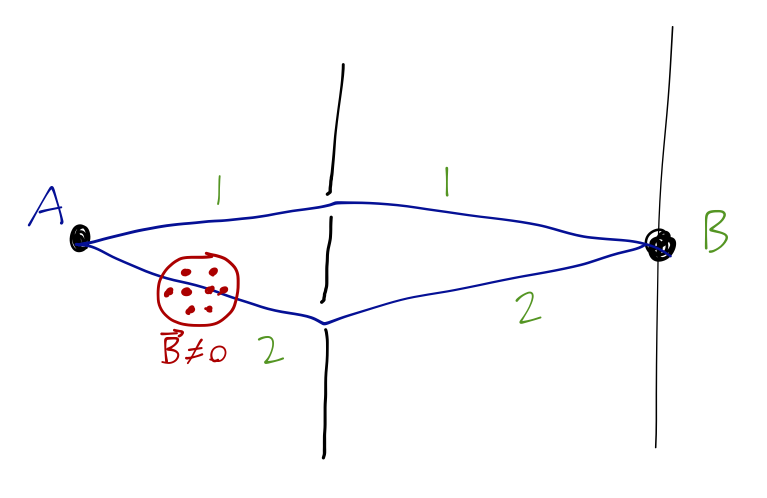
Nominally we use neutrons for this experiment, instead of electrons; neutrons also have spin-1/2 and a non-zero magnetic moment, but they don't have any charge we don't have to worry about the magnetic field significantly bending their trajectory. This is similar to the Aharonov-Bohm setup, except now we want the lower paths to always pass through a region with a magnetic field, which will shift the phase. Denoting the amplitudes for traveling from \( A \) to \( B \) on the top and bottom paths as \( A_1 \) and \( A_2 \) respectively, we see that the effect of the magnetic field will be
\[ \begin{aligned} A_2 = A_2(B=0) e^{\mp i \omega T/2}, \end{aligned} \]
where \( T \) is the time spent in the magnetic field region, and the sign ambiguity is due to the fact that the neutrons have indeterminate spin. The resulting interference term at the screen is
\[ \begin{aligned} \textrm{Re} (A_1 A_2) \sim \cos \left( \frac{\mp \omega T}{2} + \delta \right), \end{aligned} \]
where \( \delta \) is the phase shift when \( B=0 \). If we keep the time-of-flight in the magnetic field region fixed and vary \( \omega \), then we can change the interference term and thus the observed beam intensity; and the required change in order to give the same intensity back is
\[ \begin{aligned} \Delta \omega = \frac{4\pi}{T}. \end{aligned} \]
This is exactly the \( 4\pi \) we were looking for, and it has been seen conclusively in several experiments, another strong confirmation of quantum mechanics.
Next time: a little more on spin-1/2, and then we confront what happens when spin and orbital angular momentum appear together.