Last time, we ended talking about spin-1/2 particles and discovered that the spin transforms under rotations in an unfamiliar way: spin-1/2 states are \( 4\pi \) periodic rather than \( 2\pi \). This is due to the fact that a spin-1/2 "spinor", which has two components, is not quite the same as an ordinary three-component vector.
Scattering particles with spin
Scattering experiments provide a more direct way to look at the angular properties of a particle, and to see that a spin-1/2 particle is something entirely new. We consider a double-scattering experiment, involving a series of spherically symmetric targets.
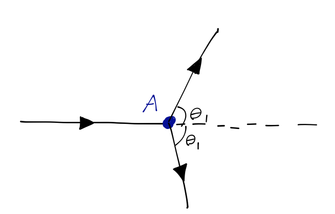
In this experiment, an incident beam of particles hits target \( A \). We haven't studied scattering theory in higher dimensions, but I will tell you that in this simple experiment, the intensity of the scattered beam is predicted to be dependent only on the angle \( \theta_1 \) between the incident and deflected beams in the beam-target plane. (This might not be completely obvious, but you can think of this as a version of the two-body problem in classical mechanics, where by symmetry we can consider the "orbits" as being confined to a plane containing the two objects.)
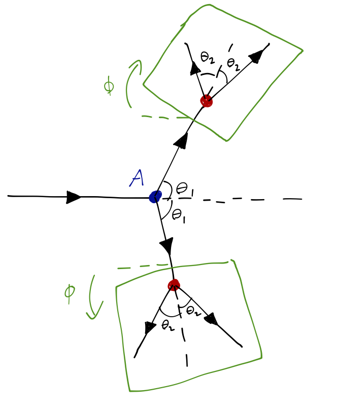
Now we introduce a pair of additional targets \( B \) and \( B' \), and we look for scattering in a second plane, which is tilted relative to the original scattering plane by an angle \( \phi \). Once again, both classically or for quantum particles which don't carry any spin, we find that the intensity of the doubly-scattered beam only depends on the angle \( \theta_2 \) in the second plane, and on the original angle \( \theta_1 \), but not on the relative orientation \( \phi \) of the two planes.
However, if the experiment is done with x-rays, then the outcome is very different. The x-ray intensity is observed to depend additionally on the orientation angle \( \phi \), proportional to \( \cos^2 \phi \). This is a polarization effect, and it's consistent with our interpretation of light as a transverse propagating wave in the vector-valued \( \vec{E} \) and \( \vec{B} \) fields. The first scattering event polarizes the light in the beam-\( A \) plane, and then the amplitude to scatter again at \( B \) or \( B' \) depends on the projection of that polarization vector onto the new scattering plane, which goes as \( \cos \phi \). Finally, the intensity is given by the squared amplitude, hence \( \cos^2 \phi \).
Finally, we repeat the experiment with a beam of electrons, protons, neutrons, etc. This time, we find an intermediate result: the doubly-scattered beam intensity goes like \( \cos \phi \). This is partly a surprise because it reveals that electron beams also exhibit some sort of polarization effect; they cannot be completely described by a scalar wavefunction \( \psi(\vec{x}) \)! (This was true of light in the previous example too, incidentally.) But this is an even stranger result, because apparently the electron wavefunction can't be represented by an ordinary vector, either; the linear dependence on \( \cos \phi \) means that the wavefunction, which we have to square to get the intensity, can't be vector-valued.
Of course, we've already seen some facets of what's going on here. An electron is a spin-1/2 particle, and it has two orthogonal spin states in addition to the spatial part of its wavefunction. We could represent its wavefunction as a two-component "column vector", but we use the word cautiously, since this is not a spatial vector; vectors in space must have three components. The two-component representation of an electron is an example of an object known as a spinor, which transforms differently from a vector. (For example, as we've seen a spinor has to be rotated around by \( 4\pi \) to return to its initial state.)
Addition of angular momentum
Despite their important differences, there is a fundamental similarity between spin and orbital angular momentum: they are both the infinitesmal generators of the rotation operator. The difference is that now we have to consider simultaneous rotation acting on two very different spaces; the infinite-dimensional position state, and the finite-dimensional space of spin states. We have a physical sense that these two spaces should be distinct in some sense, unless there is some interaction that couples them; the motion of the particle moving freely through space shouldn't care whether it is internally spin-up or spin-down.
We'll use the formerly introduced notion of a direct product to describe this system, dividing the Hilbert space into position times spin, with eigenkets \( \ket{\vec{x}} \otimes \ket{s} \). When we act with rotation by \( \phi \) around some axis \( \vec{n} \), we can write the operator on the product space as
\[ \begin{aligned} \mathcal{D}(R) = \exp \left( \frac{-i (\hat{\vec{L}} \cdot \vec{n}) \phi}{\hbar} \right) \otimes \exp \left( \frac{-i (\hat{\vec{S}} \cdot \vec{n}) \phi}{\hbar} \right). \end{aligned} \]
Now, we can write this more compactly by defining a total angular momentum operator, which combines the angular momentum operators acting on the spin and orbital parts, as
\[ \begin{aligned} \hat{\vec{J}} = \hat{\vec{L}} \otimes \hat{1} + \hat{1} \otimes \hat{\vec{S}}. \end{aligned} \]
For clarity, we'll usually assume we know how to separate the subspaces and just write \( \hat{\vec{J}} = \hat{\vec{L}} + \hat{\vec{S}} \). If we write the total rotation operator in terms of \( \hat{\vec{J}} \), we will find that it immediately splits due to the direct product into exactly the required rotation matrices using \( \hat{\vec{L}} \) and \( \hat{\vec{S}} \).
How does writing such a total angular momentum operator for such a system help? There will often be physical systems in which only the total angular momentum of a closed system is conserved, but interactions internal to the system between different types of angular momentum can occur. For example, interactions between two spin-1/2 particles may result in changes in the individual spins, but total spin should still be conserved with no external forces. Another famous and common example: the electron in a hydrogen atom has a "spin-orbit" coupling \( \hat{\vec{L}} \cdot \hat{\vec{S}} \), so \( L \) and \( S \) aren't conserved, but the total angular momentum still has to be.
We'll see explicitly how all of this works, but first let's develop some formalism related to addition of angular momentum. Suppose we have a system with two angular momentum operators, \( \hat{\vec{J}}_1 \) and \( \hat{\vec{J}}_2 \), acting on different subspaces. Individually, these operators satisfy the usual commutation relations,
\[ \begin{aligned} [\hat{J}_{1i}, \hat{J}_{1j}] = i\hbar \epsilon_{ijk} \hat{J}_{1k}, \end{aligned} \]
and the same for the components of \( \hat{\vec{J}}_2 \). Since they act on different subspaces of our Hilbert space, the operators commute with each other:
\[ \begin{aligned} [\hat{J}_{1i}, \hat{J}_{2j}] = 0. \end{aligned} \]
An arbitrary rotation generated by these two angular momentum operators acts separately on the two subspaces, but with the same axis of rotation \( \vec{n} \) and same spatial angle \( \phi \):
\[ \begin{aligned} \mathcal{D}(R) = \mathcal{D}_1(R) \otimes \mathcal{D}_2(R) = \exp \left( \frac{-i (\hat{\vec{J}}_1 \cdot \vec{n}) \phi}{\hbar} \right) \otimes \exp \left( \frac{-i (\hat{\vec{J}}_2 \cdot \vec{n}) \phi}{\hbar} \right) \end{aligned} \]
Now, we can define a total angular-momentum operator,
\[ \begin{aligned} \hat{\vec{J}} = \hat{\vec{J}}_1 + \hat{\vec{J}}_2 \end{aligned} \]
where from here on I will be implicit about the direct products, and just implicitly keep track of how things act on different subspaces. (Strictly speaking, I should have written the above as \( \hat{\vec{J}} = \hat{\vec{J}}_1 \otimes \hat{1} + \hat{1} \otimes \hat{\vec{J}}_2 \), for example.) Because \( \hat{\vec{J}}_1 \) and \( \hat{\vec{J}}_2 \) independently satisfy the angular momentum commutation relations and they commute with each other, it's easy to see that
\[ \begin{aligned} [\hat{J}_i, \hat{J}_j] = i\hbar \epsilon_{ijk} \hat{J}_k \end{aligned} \]
This makes physical sense; by way of the rotation formula I wrote above, we can think of \( \hat{\vec{J}} \) as being the generator of rotations for both subspaces \( 1 \) and \( 2 \) at once.
What do the eigenkets of this combined system look like? We already know that for an individual angular momentum operator, we typically use \( \hat{\vec{J}}^2 \) and \( \hat{J}_z \) as a CSCO, labelling our eigenkets with their respective quantum numbers \( \ket{jm} \). Clearly, one possible choice for this system is just to use this basis for both subspaces, i.e. we take the CSCO
\[ \begin{aligned} \textrm{CSCO:}\ \ \{ \hat{\vec{J}}_1{}^2, \hat{\vec{J}}_2{}^2, \hat{J}_{1,z}, \hat{J}_{2,z} \}, \end{aligned} \]
and the eigenkets are then labelled \( \ket{j_1 j_2; m_1 m_2} \). This is always a valid way to label the angular-momentum eigenkets, but as we observed before, for certain kinds of interactions we won't be able to include the Hamiltonian in our CSCO, and thus solving for the time-evolution will be complicated in this basis. In those cases, we'd much rather build a CSCO up using the total angular momentum operator \( \hat{\vec{J}} \).
Let's start with the standard choice \( \hat{\vec{J}}^2, \hat{J}_z \) to start our new CSCO. What other operators will commute with these two? We can immediately see that any of the x- or y-component operators won't work, since they won't commute with \( \hat{J}z \). What about \( \hat{J}{1z} \) or \( \hat{J}_{2z} \)? We can rewrite the operator \( \hat{\vec{J}}^2 \) in terms of the individual operators:
\[ \begin{aligned} \hat{\vec{J}}^2 = (\hat{\vec{J}}_1 + \hat{\vec{J}}_2)^2 \\ = \hat{\vec{J}}_1{}^2 + \hat{\vec{J}}_2{}^2 + 2 (\hat{\vec{J}}_1 \cdot \hat{\vec{J}}_2) \\ = \hat{\vec{J}}_1{}^2 + \hat{\vec{J}}_2{}^2 + 2 \hat{J}_{1z} \hat{J}_{2z} + \hat{J}_{1+} \hat{J}_{2-} + \hat{J}_{1-} \hat{J}_{2+}. \end{aligned} \]
The first three terms commute with either of the individual z-component operators, but the last two do not: thus \( [\hat{\vec{J}}^2, \hat{J}{1z}] \neq 0 \), and \( [\hat{\vec{J}}^2, \hat{J}{2z}] \neq 0 \). However, both \( \hat{\vec{J}}_1^2 \) and \( \hat{\vec{J}}_2^2 \) do commute with this operator, and also with \( \hat{J}z = \hat{J}{1z} + \hat{J}_{2z} \). Thus, an alternate CSCO is given by
\[ \begin{aligned} \textrm{CSCO 2:}\ \ \{ \hat{\vec{J}}{}^2, \hat{J}_z, \hat{\vec{J}}_1{}^2, \hat{\vec{J}}_2{}^2 \}. \end{aligned} \]
Using this different set of commuting operators amounts to a change of basis; in this basis, we label the eigenkets as \( \ket{j_1 j_2; j m} \). Two of the labels are the same; we've traded \( m_1 \) and \( m_2 \) for \( j \) and \( m \). Just to belabor the point, the action of the operators in our second CSCO is given by
\[ \begin{aligned} \hat{\vec{J}}_1{}^2 \ket{j_1 j_2; j m} = \hbar^2 j_1 (j_1+1) \ket{j_1 j_2; jm} \\ \hat{\vec{J}}_2{}^2 \ket{j_1 j_2; j m} = \hbar^2 j_2 (j_2 + 1) \ket{j_1 j_2; jm} \\ \hat{\vec{J}}{}^2 \ket{j_1 j_2; j m} = \hbar^2 j (j+1) \ket{j_1 j_2; jm} \\ \hat{J}_z \ket{j_1 j_2; j m} = \hbar m \ket{j_1 j_2; j m}. \end{aligned} \]
Incidentally, we used an identity above to rewrite the dot product between our two angular momenta,
\[ \begin{aligned} \hat{\vec{J}}_1 \cdot \hat{\vec{J}}_2 = \hat{J}_{1z} \hat{J}_{2z} + \frac{1}{2} (\hat{J}_{1+} \hat{J}_{2-} + \hat{J}_{1-} \hat{J}_{2+}). \end{aligned} \]
Notice how much simpler the same identity is if we work in the total angular momentum basis:
\[ \begin{aligned} 2\hat{\vec{J}}_1 \cdot \hat{\vec{J}}_2 = \hat{\vec{J}}{}^2 - \hat{\vec{J}}_1{}^2 - \hat{\vec{J}}_2{}^2. \end{aligned} \]
This way of writing the dot-product operator out is already diagonal in the eigenkets \( \ket{j_1 j_2; j m} \)! You can see now why the total angular momentum basis is strongly preferred whenever we find dot products of angular momenta in our Hamiltonian.
Clebsch-Gordan coefficients
Since the difference between our choices of CSCO is a change of basis, we know that we can write down a unitary transformation relating one basis to another, just by inserting a complete set of states:
\[ \begin{aligned} \ket{j_1 j_2; j m} = \sum_{m_1} \sum_{m_2} \ket{j_1 j_2; m_1 m_2} \sprod{j_1 j_2; m_1 m_2}{j_1 j_2; j m}. \end{aligned} \]
The components of the transformation matrix, i.e. the inner products appearing above, are known as Clebsch-Gordan coefficients, and they are of enormous importance whenever we want to study systems with multiple angular momentum operators.
Let's start by working out a few general properties of Clebsch-Gordan coefficients; we can gain some insight by acting with particular combinations of operators. For example, we have the identity
\[ \begin{aligned} (\hat{J}_z - \hat{J}_{1z} - \hat{J}_{2z}) \ket{j_1 j_2; j m} = 0, \end{aligned} \]
which holds for any ket since the combination of operators here gives the null operator. If we multiply on the left with a state in the "product basis", we have
\[ \begin{aligned} \bra{j_1 j_2; m_1 m_2} (\hat{J}_z - \hat{J}_{1z} - \hat{J}_{2z}) \ket{j_1 j_2; j m} = (m - m_1 - m_2) \sprod{j_1 j_2; m_1 m_2}{j_1 j_2; j m} = 0. \end{aligned} \]
Thus, the Clebsch-Gordan coefficients always vanish unless the eigenvalues satisfy the condition
\[ \begin{aligned} m = m_1 + m_2. \end{aligned} \]
A somewhat more difficult property to prove is the restriction on the eigenvalue \( j \):
\[ \begin{aligned} |j_1 - j_2| \leq j \leq j_1 + j_2. \end{aligned} \]
If we think of \( \hat{\vec{J}} \) as a vector sum of the individual total angular momentum operators, then this makes perfect sense, but these are operators and not just normal vectors. The proof of this relation is recursive and not very enlightening, but it's in appendix C of Sakurai if you're interested. We can further convince ourselves this has to be true just by counting up all of the eigenstates; we know that the dimension of our Hilbert space has to be the same when we change basis, so we should get the same answer. In the product basis, we know that there are \( (2j_i + 1) \) possible \( m_i \) eigenvalues, so the number of states is
\[ \begin{aligned} N = (2j_1 + 1)(2j_2 + 1). \end{aligned} \]
In the total angular momentum basis, we have \( (2j+1) \) states for each value of \( j \) allowed:
\[ \begin{aligned} N = \sum_{j=j_{min}}^{j_{max}} (2j+1) = j_{max} (j_{max} + 1) - j_{min} (j_{min} - 1) + (j_{max} - j_{min} + 1) \\ = (j_{max} + j_{min} + 1) (j_{max} - j_{min} + 1) \end{aligned} \]
which is clearly equal if we make the choices for \( j_{min} \) and \( j_{max} \) given above.
Before we go further with generalities, it's useful to see the a simple (and useful!) example: the combination of spin and angular momentum for a spin-1/2 particle.
Example: energy splittings for \( 2p \) hydrogen
As our first application of this machinery, let's study the energy levels of hydrogen for the \( 2p \) orbital (this is p-wave so \( l=1 \), and of course \( s=1/2 \)). The first correction to consider is the spin-orbit coupling,
\[ \begin{aligned} \hat{H}_{so} = f(r) \hat{\vec{S}} \cdot \hat{\vec{L}}. \end{aligned} \]
where our two angular momentum operators are the electron spin, \( \hat{\vec{S}} \), and its orbital angular momentum, \( \hat{\vec{L}} \). You can look up what \( f(r) \) actually is in a textbook - it's a combination of a bunch of constants and a \( 1/r^3 \) dependence - but it doesn't really matter for how we treat the spin-orbit interaction (except that it will reappear in an integral at the end.)
Since we've specified a p-wave orbital, we have \( l=1 \) and of course \( s=1/2 \). There are six possible states \( \ket{l, s; m_l, m_s} \) that we can write down in the product basis:
\[ \begin{aligned} \ket{1, 1/2; 1, 1/2},\ \ \ \ket{1, 1/2; 1, -1/2}, \\ \ket{1, 1/2; 0, 1/2},\ \ \ \ket{1, 1/2; 0, -1/2}, \\ \ket{1, 1/2; -1, 1/2},\ \ \ \ket{1, 1/2; -1, -1/2}. \end{aligned} \]
Now, we can just apply the operator \( \hat{\vec{S}} \cdot \hat{\vec{L}} \) to these states directly; they're not eigenstates of that operator (since it contains the \( x \) and \( y \) components of both angular momenta), but we know how to evaluate them. However, the operators we're using in our CSCO here don't commute with \( \hat{\vec{S}} \cdot \hat{\vec{L}} \) and thus don't commute with \( \hat{H} \), so finding energy eigenvalues/eigenstates will be a pain. On the other hand, since
\[ \begin{aligned} \hat{\vec{S}} \cdot \hat{\vec{L}} = (\hat{\vec{S}} + \hat{\vec{L}})^2 - \hat{\vec{S}}{}^2 - \hat{\vec{L}}{}^2 \\ = \frac{1}{2} (\hat{\vec{J}}{}^2 - \hat{\vec{L}}{}^2 - \hat{\vec{S}}{}^2), \end{aligned} \]
working in the total angular momentum basis \( \ket{1, 1/2; j,m} \) will simplify things for us. I'm going to drop the first two labels from all of our kets, since they're always just \( 1 \) and \( 1/2 \) here. To switch basis, our new states are given by the formula
\[ \begin{aligned} \ket{j,m} = \sum_{m_l} \sum_{m_s} \ket{\ell, s; m_l, m_s} \sprod{\ell, s; m_l, m_s}{j,m} \end{aligned} \]
so now we just need to calculate these inner products (a.k.a. the Clebsch-Gordan coefficients.) By the way, I will keep the total angular momentum eigenvalues to label the product-basis states, but drop them in the total basis states, just to help us keep track of which is which.
Actually, before we get to Clebsch-Gordan, we can already notice that the action of the spin-orbit coupling on total angular momentum basis states is nice and simple:
\[ \begin{aligned} \hat{H}_{so} \ket{j, m} = \frac{1}{2} \hbar^2 f(r) (j(j+1) - l(l+1) - s(s+1)) \ket{j, m}. \end{aligned} \]
This depends only on \( j \) and not \( m \), so we have two distinct spin-orbit eigenvalues
\[ \begin{aligned} \hat{H}_{so} \ket{1/2, m} = -\hbar^2 f(r) \ket{1/2, m} \\ \hat{H}_{so} \ket{3/2, m} = \frac{1}{2} \hbar^2 f(r) \ket{3/2, m}. \end{aligned} \]
In principle, the spin-orbit coupling modifies the Schrödinger equation itself, so we'd have to (re-)solve the hydrogen atom at this point. But the spin-orbit coupling is rather small, so I will instead invoke a result from perturbation theory: we can approximate the energy shift by calculating the expectation value of the perturbation Hamiltonian in terms of the old eigenstates,
\[ \begin{aligned} E_{so} \approx \bra{j,m} \hat{H}_{so} \ket{j,m}. \end{aligned} \]
We'll prove this result later on, but for now just take my word for it. There is still some radial dependence to deal with, but that means just have to average over the radial wavefunction as part of the expectation value:
\[ \begin{aligned} E_{so,j} = \int_0^\infty dr\ r^2 |R_{nl}(r)|^2 f(r)\ \bra{j, m} \hat{\vec{S}} \cdot \hat{\vec{L}} \ket{j,m}, \end{aligned} \]
where \( R_{nl}(r) \) are the standard radial wavefunctions for hydrogen. I'll skip the actual details of this integral, but the result for \( 2p \) hydrogen turns out to be quite small, with the spin-orbit splitting on the order of \( 5 \times 10^{-5} \) eV. Even without the integral, we have obtained the qualitative result that the \( 2p \) energy level splits apart into two energy levels with \( j=1/2 \) and \( j=3/2 \); furthermore, the \( j=1/2 \) splitting is negative, so it is the lower energy level.
A brief aside on notation: with the inclusion of orbital angular momentum, it's no longer sufficient for us to use the ordinary spectroscopic notation \( (s,p,d,f,...) \) that we introduced before. For example, the spin-1/2 electron in an \( l=1 \) orbital has two distinct energy levels, corresponding to \( j=1/2 \) and \( j=3/2 \). To deal with systems containing combinations of spin and angular momentum, we introduce the modified spectroscopic notation, which looks like this:
\[ \begin{aligned} {}^{2S+1} L_J \end{aligned} \]
Here \( L \) is the orbital angular momentum quantum number, which we now write as a capital letter: \( l=0 \) becomes \( S \), \( l=1 \) is \( P \), and so on. \( S \) is the spin quantum number, so \( 2S+1 \) labels the number of degenerate spin states. The two states we encountered in our example last time were thus \( ^{2}P_{1/2} \) and \( ^{2}P_{3/2} \).
A state with no angular momentum and no spin would be \( ^{1}S_0 \). This isn't as trivial as it looks; in fact, such a spectroscopic label occurs very frequently in atoms with multiple electrons. The ground state of helium, and indeed of each of the noble gases, is labeled \( ^{1}S_0 \).
If we consider this effect together with the \( 2s \) energy level which has no spin-orbit term, we could sketch an energy splitting diagram like the following:
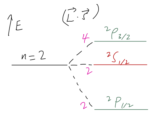
(Here I've labelled the degeneracy of each state in magenta along the splitting lines.) I should point out that this is qualitatively right, but for the wrong reason; in the real world there are other effects in hydrogen of the same order of magnitude that contribute to the splittings between these three spectroscopic levels. We may see them in detail at the end of the semester.
Next time: we see what Clebsch-Gordan coefficients are good for.