Last time, we were studying the effect of the spin-orbit coupling in \( 2p \) hydrogen, and found the following qualitative result:
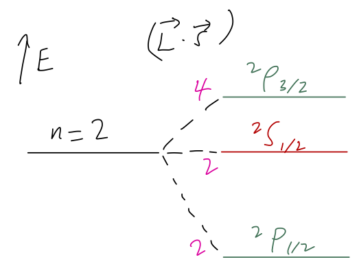
(Here I've labelled the degeneracy of each state in magenta along the splitting lines.) I should point out that this is qualitatively right, but for the wrong reason; in the real world there are other effects in hydrogen of the same order of magnitude that contribute to the splittings between these three spectroscopic levels. We may see them in detail at the end of the semester. (Actually, the \( ^2S_{1/2} \) state is much closer to the \( ^2P_{1/2} \) state, due to some of these other effects.)
So what's the use of Clebsch-Gordan coefficients, then? Since they give us a change of basis, they're really crucial in situations when we need to use both bases at once. An example would be if we apply a weak magnetic field to the 2p hydrogen atom, which gives another contribution to the Hamiltonian of the form
\[ \begin{aligned} \hat{H}_B = \mu_B B (\hat{L}_z + 2 \hat{S}_z). \end{aligned} \]
This cannot be easily written in terms of the total angular momentum; but if we have the Clebsch-Gordan coefficients, we can use the separate angular momentum eigenbasis at the same time.
Let's begin working out the change of basis. Remembering the general rules we derived for the C-G coefficients, we start by noting that \( m = m_l + m_s \), which immediately tells us that \( -3/2 \leq m \leq 3/2 \). We also have from the triangle inequality \( 1/2 \leq j \leq 3/2 \).
Just to check ourselves, notice that the counting of states here makes sense. There are six states we can write down in the total basis based on the above restrictions:
\[ \begin{aligned} \ket{3/2, 3/2}, \\ \ket{3/2, 1/2}, \ \ \ \ket{1/2, 1/2}, \\ \ket{3/2, -1/2}, \ \ \ \ket{1/2, -1/2}, \\ \ket{3/2, -3/2}. \end{aligned} \]
We can now demonstrate a general procedure for finding the C-G coefficients (although this is not an efficient procedure, especially for higher angular momentum; if you are dealing professionally with Clebsch-Gordan coefficients, you will probably use pre-calculated tables or computer packages.)
We begin "at the top", with the state with maximum \( m \), \( \ket{3/2, 3/2} \). Since there is only one product-basis state satisfying \( m_l + m_s = 3/2 \), the sum
\[ \begin{aligned} \ket{j_1 j_2; j m} = \sum_{m_1} \sum_{m_2} \ket{j_1 j_2; m_1 m_2} \sprod{j_1 j_2; m_1 m_2}{j_1 j_2; j m}. \end{aligned} \]
has only one term:
\[ \begin{aligned} \ket{3/2, 3/2} = \ket{1, 1/2; 1, 1/2} \sprod{1, 1/2; 1, 1/2}{3/2,3/2}. \end{aligned} \]
Since we assume the original state is already normalized, the Clebsch-Gordan coefficient appearing here must simply be \( 1 \).
Moving on to \( \ket{3/2, 1/2} \), there are two states in the original basis that will contribute, so we can't make such a simple argument. However, since we already have one state in the new basis, we can just use the ladder operators to derive other states. The ladder operators in the total angular momentum basis are just
\[ \begin{aligned} \hat{J}_{\pm} = \hat{L}_{\pm} + \hat{S}_{\pm} \end{aligned} \]
This is a good time to remind ourselves that the ladder operators act like so:
\[ \begin{aligned} \hat{J}_{\pm} \ket{j, m} = \hbar \sqrt{(j \mp m) (j \pm m + 1)} \ket{j, m \pm 1}. \end{aligned} \]
Now, acting on the total-basis state, we have
\[ \begin{aligned} \hat{J}_- \ket{3/2, 3/2} = \sqrt{3} \hbar \ket{3/2, 1/2}. \end{aligned} \]
But from the definition above, we can also write
\[ \begin{aligned} \hat{J}_- \ket{3/2, 3/2} = (\hat{L}_- + \hat{S}_-) \ket{1, 1/2; 1, 1/2} \\ = \hbar \sqrt{2} \ket{1, 1/2; 0, 1/2} + \hbar \ket{1, 1/2; 1, -1/2}. \\ \end{aligned} \]
Thus, the total-basis state is given in terms of the product basis by
\[ \begin{aligned} \ket{3/2, 1/2} = \sqrt{\frac{2}{3}} \ket{1, 1/2; 0, 1/2} + \sqrt{\frac{1}{3}} \ket{1, 1/2; 1, -1/2}. \end{aligned} \]
As a check, we notice that this state is properly normalized, since the squared coefficients add to 1. To get \( \ket{3/2, -1/2} \), we can just apply the lowering operator again, and then again to get \( \ket{3/2, -3/2} \), but let me come back to those; there's a nice symmetry-based way to get them instead of just grinding through ladder operators.
This leaves us with two states to find; the pair of \( j=1/2 \) states. They will each overlap with two of the product-basis states, so we don't have a nice starting point for the use of ladder operators anymore. However, we can still use the ladder operators to make progress. If we try to raise the state \( \ket{1/2, 1/2} \), we know we should get zero, so:
\[ \begin{aligned} \hat{J}_+ \ket{1/2, 1/2} = 0 = (\hat{L}_+ + \hat{S}_+) \left( \alpha \ket{1, 1/2; 1, -1/2} + \beta \ket{1, 1/2; 0, 1/2} \right) \\ = \hbar \alpha \ket{1, 1/2; 1, 1/2} + \sqrt{2} \hbar \beta \ket{1, 1/2; 1, 1/2}. \end{aligned} \]
So \( \alpha + \sqrt{2} \beta = 0 \), and the state must also be properly normalized, so \( \alpha^2 + \beta^2 = 1 \). This is all we need to solve for the coefficients: we can rewrite the first equation in the form \( \alpha^2 - 2\beta^2 = 0 \), and then the solution is easy:
\[ \begin{aligned} \ket{1/2, 1/2} = \sqrt{\frac{2}{3}} \ket{1, 1/2; 1, -1/2} - \sqrt{\frac{1}{3}} \ket{1, 1/2; 0, 1/2}. \end{aligned} \]
The sign ensures that this state is orthogonal to the similar-looking \( \ket{3/2, 1/2} \) state; in fact, we could have solved for these coefficients just by requiring orthogonality in this case. The last state \( \ket{1/2, -1/2} \) can then be found using the lowering operator on \( \ket{1/2, 1/2} \) once more.
Clebsch-Gordan phase conventions and recursion relations
Note that there is an overall sign ambiguity above; we could have instead chosen \( \alpha \) to be negative and \( \beta \) positive. This is secretly present even before we get to this point; even insisting that our Clebsch-Gordan coefficients all be real, we could have taken \( (-1) \) instead of \( (+1) \) times the product-basis states for the \( m=\pm 3/2 \) states. The standard sign convention for the C-G coefficients, and the one we will follow, is that the overlap between the highest components of \( \hat{\vec{J}}_1 \) and \( \hat{\vec{J}} \) is always positive, i.e.
\[ \begin{aligned} \sprod{j_1 j_2; j j}{j_1 j_2; j_1 m_2} > 0. \end{aligned} \]
In our \( 2p \) hydrogen example, this gives the conditions
\[ \begin{aligned} \sprod{3/2, 3/2}{1, 1/2; 1, 1/2} > 0,\\ \sprod{1/2,1/2}{1, 1/2; 1, -1/2} > 0. \end{aligned} \]
This immediately forces some other states to have minus signs, as dictated by the equations obtained from raising and lowering operators. To see why, let's make a slight detour and write down a general recursion relation for the Clebsch-Gordan coefficients. All we're going to do is write out the same raising and lowering operator equation, but now for a totally general combination of states. Start by applying the ladder operators in the total basis:
\[ \begin{aligned} \hat{J}_{\pm} \ket{j_1, j_2; j, m} = \hbar \sqrt{(j \mp m)(j \pm m + 1)} \ket{j_1, j_2; j, m \pm 1}. \end{aligned} \]
On the other side, we write out the state in the product basis:
\[ \begin{aligned} \hat{J}_{\pm} (\ket{j_1, j_2; j, m} = (\hat{J}_{1, \pm} + \hat{J}_{2, \pm}) \sum_{m_1', m_2'} \ket{j_1, j_2; m_1', m_2'} \sprod{j_1, j_2; m_1', m_2'}{j_1, j_2; j, m} \\ = \hbar \sum_{m_1', m_2'} \left[ \sqrt{j_1 \mp m_1')(j_1 \pm m_1' + 1)} \ket{j_1, j_2; m_1' \pm 1, m_2'} \right. \\ \left. + \sqrt{(j_2 \mp m_2')(j_2 \pm m_2' + 1)} \ket{j_1, j_2; m_1', m_2' \pm 1}\right] \sprod{j_1, j_2; m_1', m_2'}{j_1, j_2; j, m}. \end{aligned} \]
This is a big, messy sum, but of course many of the terms are automatically zero. If we'd like to isolate a particular Clebsch-Gordan coefficient, we multiply both sides on the left by \( \bra{j_1, j_2; m_1, m_2} \), and the sums on the right collapse, leaving only the terms satisfying either
\[ \begin{aligned} m_1' = m_1 \mp 1,\ \ m_2' = m_2 \end{aligned} \]
or
\[ \begin{aligned} m_1' = m_1,\ \ m_2' = m_2 \mp 1. \end{aligned} \]
The result is the recursion identity:
\[ \begin{aligned} \sqrt{(j \mp m)(j \pm m + 1)} \sprod{j_1, j_2; m_1, m_2}{j, m \pm 1} \\ = \sqrt{(j_1 \pm m_1)(j_1 \mp m_1 + 1)} \sprod{j_1, j_2; m_1 \mp 1, m_2}{j, m} + \\ \sqrt{(j_2 \pm m_2)(j_2 \mp m_2 + 1)} \sprod{j_1, j_2; m_1, m_2 \mp 1}{j,m}, \end{aligned} \]
where you should be careful with the signs! Now, if we set \( m=j \) and apply the raising operator, the left-hand side vanishes, and we find the relation
\[ \begin{aligned} \sprod{j_1, j_2; m_1 -1, m_2}{j, j} = -\sqrt{\frac{(j_2 + m_2)(j_2 - m_2 +1)}{(j_1 + m_1)(j_1 - m_1 + 1)}} \sprod{j_1, j_2; m_1, m_2 - 1}{j, j}. \end{aligned} \]
Once again, our phase convention is to take the sign of the coefficient with highest \( m \) for the first angular momentum, i.e. \( m_1 = j_1 \) and \( m_2 = j - j_2 \), to be positive. Applying the above formula recursively then gives us the sign of other C-G coefficients. Incidentally, this also ensures that all of the C-G coefficients in this series are real, once we've set the first coefficient to \( 1 \). It's important to note also that this only fixes the signs of some of the coefficients; for an arbitrary choice of \( m_1, m_2, m \), the sign isn't so easy to predict.
One subtlety of this phase convention is that it matters which angular momentum we call "first" and which one is "second". If we swap them around, then the Clebsch-Gordan coefficients pick up another sign according to the relation
\[ \begin{aligned} \sprod{j_1 j_2; jm}{j_1 j_2; m_1 m_2} = (-1)^{j-j_1-j_2} \sprod{j_2 j_1; jm}{j_2 j_1; m_2 m_1}. \end{aligned} \]
Finally, if you look up a table of Clebsch-Gordan coefficients, you will often see the coefficients printed only for \( m \geq 0 \). This is because of another symmetry of the C-G coefficients:
\[ \begin{aligned} \sprod{j_1, j_2; j, -m}{j_1, j_2; -m_1, -m_2} = (-1)^{j-j_1-j_2} \sprod{j_1, j_2; j, m}{j_1, j_2; m_1, m_2}. \end{aligned} \]
I won't prove this one in detail, but the argument involves starting with the lowest state \( \ket{j, -j} \) and using raising operators; as always the sign arises from our phase convention involving the "highest" state \( \ket{j, j} \).
Let's recollect what we found above. For the three states with \( m \geq 0 \), we have
\[ \begin{aligned} \ket{3/2, 3/2} = \ket{1, 1/2; 1, 1/2} \\ \ket{3/2, 1/2} = \sqrt{\frac{2}{3}} \ket{1, 1/2; 0, 1/2} + \sqrt{\frac{1}{3}} \ket{1, 1/2; 1, -1/2} \\ \ket{1/2, 1/2} = \sqrt{\frac{2}{3}} \ket{1, 1/2; 1, -1/2} - \sqrt{\frac{1}{3}} \ket{1, 1/2; 0, 1/2}. \end{aligned} \]
The other three are given by the symmetry formula above, where we can flip all of the signs \( m, m_1, m_2 \) and pick up an overall sign \( (-1)^{j-j_1-j_2} = (-1)^{j-3/2} \). For example, we have
\[ \begin{aligned} \ket{3/2, -1/2} = \sprod{1,1/2; -1, 1/2}{3/2, -1/2} \ket{1, 1/2; -1, 1/2} + \sprod{1,1/2; 0, -1/2}{3/2, -1/2} \ket{1, 1/2; 0, -1/2} \\ = \sprod{1,1/2; 1, -1/2}{3/2, 1/2} \ket{1, 1/2; -1, 1/2} + \sprod{1,1/2;0,1/2}{3/2, 1/2} \ket{1, 1/2; 0, -1/2} \\ = \sqrt{\frac{1}{3}} \ket{1, 1/2; -1, 1/2} + \sqrt{\frac{2}{3}} \ket{1, 1/2; 0, -1/2}. \end{aligned} \]
We can write all of these coefficients more compactly as a matrix (after all, this is a unitary transformation:)
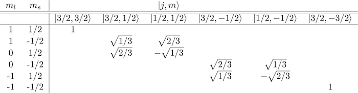
This matrix is block diagonal, with the blocks of size at most 2, due to the fact that one of the angular momenta we're adding is spin-\( 1/2 \), with only two possible states; the maximum number of solutions to \( m_l + m_s = m \) is thus two. If we add two higher spins, the blocks will be larger. All of the states are orthogonal, as they must be since we wanted to find an orthonormal basis.
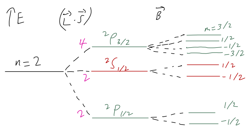
Now we return to \( 2p \) hydrogen, and adding a small applied magnetic field (on top of our spin-orbit coupling):
\[ \begin{aligned} \hat{H}_B = \mu_B B (\hat{L}_z + 2 \hat{S}_z) \end{aligned} \]
Once again, I'll invoke the result from perturbation theory that for sufficiently small \( B \), we have for the energy shift
\[ \begin{aligned} E_{B,j,m} \approx \bra{j,m} \mu_B B (\hat{L}_z + 2 \hat{S}_z) \ket{j,m}. \end{aligned} \]
For the highest \( j=3/2 \) state, rewriting in the product basis is easy:
\[ \begin{aligned} E_{B,3/2,3/2} \approx \mu_B B \bra{1,1/2; 1,1/2} (\hat{L}_z + 2\hat{S}_z) \ket{1,1/2; 1,1/2} \\ = 2\hbar \mu_B B. \end{aligned} \]
The next lower state is harder, but not by much:
\[ \begin{aligned} E_{B,3/2,1/2} \approx \mu_B B \left( \frac{2}{3} \bra{1,1/2; 0,1/2} \hat{L}_z + 2\hat{S}_z \ket{1,1/2; 0,1/2} \right. \\ \left.+ \frac{1}{3} \bra{1,1/2;1,-1/2} \hat{L}_z + 2\hat{S}_z \ket{1,1/2; 1,-1/2} \right) \\ = \frac{2}{3} \hbar \mu_B B. \end{aligned} \]
We can keep going like this; I'll let you work out the remaining energies yourself. The general result turns out to be, compactly,
\[ \begin{aligned} E_{B,m,j} = \frac{1}{3} m (2j+1) \hbar \mu_B B. \end{aligned} \]
With the spin-orbit term, the spectral line associated with the \( 2p \) orbital of hydrogen splits according to \( j \) into two states; the addition of a small magnetic field breaks any remaining symmetry and splits all six states apart. And thanks to the formalism we've developed, we were able to easily calculate both terms, even though we had to work in two different bases to do so. Hopefully now you can appreciate the power of the Clebsch-Gordan coefficients!
We can sum up our result with the following sketch, assuming \( B \) is small enough that the magnetic splitting is smaller than the spin-orbit effect:
Total angular momentum and reducible operators
Another point worth noticing is that in the total basis, our space has split into two separate spaces with total \( j=3/2 \) and \( j=1/2 \). The raising and lowering operators \( \hat{J}_{\pm} \) do not connect these two spaces together; we can think of now having two complete Hilbert spaces in terms of \( \hat{\vec{J}} \) that don't overlap. This is in contrast to the original product basis, where we had to specify both \( m_l \) and \( m_s \). In mathematical notation, the decomposition we've just done is written in the form
\[ \begin{aligned} 1 \otimes \frac{1}{2} = \frac{3}{2} \oplus \frac{1}{2}. \end{aligned} \]
In other words, our change of basis has decomposed a direct product (in which we require information from both the left and right spaces in order to describe a particular state) to a direct sum (in which the states can be in either the left or right space.) Of course, we can have a more general state vector which is a sum of \( j=3/2 \) and \( j=1/2 \) states, it's just not an angular momentum eigenstate anymore.
Note that in terms of the dimension of these spaces, the direct product and direct sum act just like normal multiplication and addition operators, respectively. In this example, the direct product space has \( 3 \times 2 = 6 \) possible states. In the total basis, there are 4 \( j=3/2 \) states and 2 \( j=1/2 \) states, so we once again find 6 (as we must). This provides a quick cross-check of our thinking, particularly when the decompositions become more complicated. For example, for addition of two spin-1 systems we would write
\[ \begin{aligned} 1 \otimes 1 = 2 \oplus 1 \oplus 0, \end{aligned} \]
where the result of the product just follows from the rules we've already discovered for addition of angular momentum, namely \( |j_1 - j_2| \leq j \leq j_1 + j_2 \) and \( m = m_1 + m_2 \) (the latter ensuring all of the \( j,m \) values are either integer or half-integer but never both in the same expansion.) We can check by counting the dimensions of the Hilbert space: on the left we have \( 3 \times 3 \), and on the right \( 5 + 3 + 1 \).
Next time: more on this, the Wigner D-matrix, and we move towards tensor operators.