Last time, we ended by talking about reducible operators, and how going from the individual angular momentum basis to the total angular momentum basis can be viewed as going from a direct product to a direct sum. This is just another (group theoretic) way of describing a phenomenon we've already seen in detail, which is addition of angular momentum. In fact, we can write the general result of this direct product in terms of the angular momentum quantum numbers: for adding \( \hat{\vec{J}}_1 + \hat{\vec{J}}_2 \), the Hilbert space of \( \hat{\vec{J}} \) can be decomposed as
\[ \begin{aligned} j_1 \otimes j_2 = |j_1 - j_2| \oplus (|j_1 - j_2| + 1) \oplus ... \oplus (j_1 + j_2). \end{aligned} \]
This is just another way to write the selection rule giving the possible values of \( j \), which we've already seen. For those of you who haven't seen this sort of thing before, I'm going to do a little mini-review here: if you're still puzzled by what we're doing, you should have a look at these nice lecture notes from Hitoshi Murayama about tensor products.
Quick review: direct sums and tensor products
To be concrete, suppose we have two vector spaces \( V_A \) and \( V_B \), with dimensions \( m \) and \( n \). They each have a set of basis vectors \( {\hat{e}_1, ..., \hat{e}_m} \) and \( {\hat{f}_1, ..., \hat{f}_n} \). Suppose we want to combine them together to form a single vector space: how can we do it?
One possibility is to form the direct sum, \( V_A \oplus V_B \). This creates a new \( (m+n) \)-dimensional vector space with basis simply equal to the union of the two original bases, i.e.
\[ \begin{aligned} \{\hat{e}_1, ..., \hat{e}_m, \hat{f}_1, ... \hat{f}_n \}. \end{aligned} \]
If \( \vec{v} \) is a vector in \( V_A \) and \( \vec{w} \) a vector in \( V_B \), we can also define the vector direct sum \( v \oplus w \) in the obvious way: its \( m + n \) components are just given by stacking the components in each individual space. For example, if \( m=2 \) and \( n=3 \), then
\[ \begin{aligned} \vec{v} \oplus \vec{w} = \left( \begin{array}{c} v_1 \\ v_2 \\ w_1 \\ w_2 \\ w_3 \end{array} \right). \end{aligned} \]
All of our original vectors are in the new direct-sum space, e.g. for every \( \vec{v} \) in \( V_A \), we can write \( \vec{v} \oplus \vec{0} \) in \( V_A \oplus V_B \).
If \( A \) is a matrix acting on vectors in \( V_A \) and \( B \) is a matrix acting on \( V_B \), then we can combine them block-diagonally to obtain a matrix acting on \( V_A \oplus V_B \):
\[ \begin{aligned} A \oplus B = \left( \begin{array}{cc} A_{m \times m} & 0_{m \times n} \\ 0_{n \times m} & B_{n \times n} \end{array} \right). \end{aligned} \]
This doesn't imply that every matrix on the direct sum space can be written in this block-diagonal form, but we can make such a matrix from any matrices on the original spaces. When working with such composite matrices, the operations are very simple: we see that
\[ \begin{aligned} (A_1 \oplus B_1) (A_2 \oplus B_2) = (A_1 A_2) \oplus (B_1 B_2) \\ (A \oplus B) (\vec{v} \oplus \vec{w}) = (A\vec{v}) \oplus (B\vec{w}) \end{aligned} \]
i.e. all the operations just break apart into operations on our original spaces.
The other way we can form a new vector space from our original pair is by taking the direct product, \( V_A \otimes V_B \) (also known as the "tensor product".) In the direct product, we define our new basis vectors by pairing together all possible combinations of the original basis, i.e.
\[ \begin{aligned} \{\hat{e}_i \otimes \hat{f}_j\},\ \ i = 1...m,\ \ j=1...n \end{aligned} \]
This gives a space of dimension \( mn \). The "tensor" in the name is self-evident, since our basis vectors are now tensors - you can think of them as having two indices, \( i \) and \( j \).
Let's go back to our concrete example from above where \( m=2 \) and \( n=3 \). Then our direct product basis is six-dimensional: given two vectors \( \vec{v} \) and \( \vec{w} \), then their tensor product is
\[ \begin{aligned} \vec{v} \otimes \vec{w} = \left( \begin{array}{c} v_1 w_1 \\ v_1 w_2 \\ v_1 w_3 \\ v_2 w_1 \\ v_2 w_2 \\ v_2 w_3 \end{array} \right). \end{aligned} \]
For matrices, we can similarly form \( A \otimes B \), but it's not as simple as just stacking them together anymore. We define the direct product of matrices by requiring that its action on direct products of vectors decomposes over the original spaces, i.e.
\[ \begin{aligned} (A \otimes B) (\vec{v} \otimes \vec{w}) = (A\vec{v} \otimes B\vec{w}). \end{aligned} \]
The resulting matrix (which you may also hear referred to as the matrix outer product or Kronecker product) will usually be rather dense. It's easiest to see how this works if one of the matrices is the identity, e.g.
\[ \begin{aligned} A \otimes I = \left( \begin{array}{cccccc} a_{11} & 0 & 0 & a_{12} & 0 & 0 \\ 0 & a_{11} & 0 & 0 & a_{12} & 0 \\ 0 & 0 & a_{11} & 0 & 0 & a_{12} \\ a_{21} & 0 & 0 & a_{22} & 0 & 0 \\ 0 & a_{21} & 0 & 0 & a_{22} & 0 \\ 0 & 0 & a_{21} & 0 & 0 & a_{22} \end{array} \right) \end{aligned} \]
You can verify that multiplying this out gives the expected result
\[ \begin{aligned} (A \otimes I) (\vec{v} \otimes \vec{w}) = (A\vec{v}) \otimes \vec{w}. \end{aligned} \]
So in general, direct products are much more complicated to work with than direct sums; most natural matrices we build from individual spaces are not diagonal. On the other hand, direct sums give block diagonal subspaces that can easily be worked with separately. This is the power of the addition of angular momentum: for a system with multiple forms of angular momentum, rewriting in terms of the total angular momentum reveals the block diagonal (direct sum) structure!
Groups and representations
I'm going to assume you're all familiar with some amount of group theory (or at least have a rough idea of what I mean when I say "group"), but I'll do a very quick review here. A group is a collection of objects together with an operation, \( \cdot \), which satisfy the following rules:
- Closure: \( (a \cdot b) \) is still in the group
- Associativity: \( a \cdot (b \cdot c) = (a \cdot b) \cdot c \)
- Identity: the group contains 1 so that \( (1 \cdot a) = (a \cdot 1) = 1 \)
- Inverse: there is always \( a^{-1} \) so that \( a^{-1} \cdot a = a \cdot a^{-1} = 1 \).
Most mathematical spaces we're familiar with are groups. In particular, the space of (invertible) \( N \times N \) matrices (known as \( GL(N,\mathbb{C}) \) if the entries are complex) forms a group. In fact, the structure of \( GL(N,\mathbb{C}) \) is flexible enough that in most cases, if we're handed a group (list of elements and what their products are), we can represent all of the group elements as \( N \times N \) matrices.
In fact, because \( N \times N \) matrices can also serve as operators acting on a vector space, this representation is even more powerful. After all, in physics the properties of a symmetry group alone aren't nearly as useful as the properties of other objects when the symmetry acts on them.
Concretely, a representation is a map
\[ \begin{aligned} R: G \rightarrow GL(V) \end{aligned} \]
that takes elements in some group \( G \), and gives us back matrices over some vector space. Because this map is supposed to "represent" what the group does, it must preserve the group product: in other words,
\[ \begin{aligned} a \cdot b = c \Rightarrow R(a) R(b) = R(c). \end{aligned} \]
Now, the representation of a particular group is usually not unique: there can be many possible choices of different dimensions. A representation can be trivial: the map \( R(g) = 1 \) always satisfies the relationship above. But we can go further to the idea of a faithful representation, which is any \( R \) that always maps distinct elements of \( g \) to distinct matrices \( R(g) \).
Even with faithful representations, there are still many ways to construct a representation \( R \). Suppose our group is \( \mathcal{Z}_2 \), i.e. the group with two elements, \( 1 \) and \( a \) such that \( a \cdot a = 1 \). A faithful representation is obtained by mapping \( 1 \) into the identity matrix, and \( a \) into any \( N \times N \) matrix \( A \) which satisfies \( A^2 = 1 \). There are an infinite number of possibilities, and more importantly, we can do this construction for matrices of any size \( N \). A representation constructed from \( N \times N \) matrices is said to have dimension \( N \).
Tying back to what we've been talking about, since representations are maps into a vector space, we can use exactly the same notation to define direct sums and tensor products of representations. If \( R_A: G \rightarrow A \) and \( R_B: G \rightarrow B \), then \( R_A \oplus R_B: G \rightarrow A \oplus B \), and similarly for \( R_A \otimes R_B \).
So why is representation theory useful? In physics especially, we're not just interested in the structure of groups themselves; most of the groups we care about are symmetry groups, which means they also have an action associated with them, i.e. symmetry group elements act on physical objects and transform them in some way. Representation theory is a natural way to deal with this: the group elements are matrices, and the physical states etc. are vectors acted on by the matrices. An important point is that we then have to assign the physical states themselves to a particular representation; in other words, if we're representing physical states as vectors, we have to specify what dimension they are.
Rotational symmetry is actually a great example. Thinking back to classical mechanics, you know that you can describe an arbitrary rotation in terms of 3x3 rotation matrices; these matrices form a group by our rules above. Specifically, the rotation group is the "special orthogonal" group \( SO(3) \), which is the group of 3x3 matrices with \( \det R = 1 \) (special) and \( R^T R = 1 \) (orthogonal).
What's crucial to note here is that rotation symmetry is always the same group, \( SO(3) \), which is just a subset of the full Lorentz group we're about to investigate; the 3 comes from the number of spatial dimensions. However, it can act differently on different physical objects. Remembering back to classical mechanics, a position vector transforms differently from, say, the inertia tensor, which transforms differently from a scalar quantity like energy:
\[ \begin{aligned} \vec{r} \rightarrow R \vec{r} \\ I \rightarrow R^T I R \\ E \rightarrow E \end{aligned} \]
We identify each of these quantities with different representations of the rotation group. We're still using \( 3x3 \) matrices to transform the inertia tensor, but don't get misled by the notation here: under rotations, \( I \) is a nine-component object, and we could have written it as a vector which is acted on by a \( 9x9 \) rotation matrix instead to be more consistent.
By the way, a little more terminology: scalars like energy don't transform at all under rotation, so they exist in the trivial representation, which has dimension 1. Vectors transform according to 3x3 rotation matrices, so their representation is the group: this is the fundamental representation.
What about the inertia tensor? We know that it is actually defined in classical mechanics as a product of two vectors (and an integral):
\[ \begin{aligned} I_{jk} = \int dV\ \rho(\vec{r}) (r^2 \delta_{jk} - r_j r_k) \end{aligned} \]
This is an example of a dyadic tensor; it's a tensor with two vector indices. As I already noted, this transforms as a nine-dimensional representation of the rotation group. However, we know that it's formed as a direct product of two vectors, so the representation of rotations will also be a direct product. This will be a dense 9x9 matrix. But we might hope that there exists a decomposition into a direct sum.
In fact, this decomposition is exactly what is guaranteed by representation theory, and it's what we've already proved using addition of angular momentum! The decomposition in terms of the dimension of the representation is
\[ \begin{aligned} \textbf{3} \otimes \textbf{3} = \textbf{5} \oplus \textbf{3} \oplus \textbf{1} \end{aligned} \]
These latter representations are irreducible representations, which simply means they cannot be decomposed further. The general problem of finding all such decompositions and irreducible representations for a given group is known as plethysm. We only know the answer for the rotation group already because we went to a lot of trouble to solve the addition of angular momentum problem! Concretely, this decomposition means we should be able to identify three smaller components within the tensor \( I \), which transform as a scalar, as a vector, and as a five-dimensional object; we'll see concretely how this works in a little bit.
We can explicitly see the block-diagonal structure appearing if we consider how a rotation acts on our system of total angular momentum. On the homework, you explored the use of the Wigner D-matrix to describe what happens to angular momentum eigenstates under rotations:
\[ \begin{aligned} \mathcal{D}_{m'm}^{(j)}(R) = \bra{j,m'} \exp \left( \frac{-i (\hat{\vec{J}} \cdot \vec{n}) \phi}{\hbar} \right) \ket{j,m} \end{aligned} \]
When we apply a rotation to our quantum system, the Wigner D-matrix tells us the amplitude for a rotated angular momentum eigenstate \( \ket{j,m} \) to be found in another angular momentum eigenstate \( \ket{j,m'} \); by Born's rule the probability of measuring \(\hat{J}_z' = m'\) after rotation is precisely \(|\mathcal{D}_{m'm}^{(j)}(R)|^2\).
It's important to note that the same total quantum number \( j \) appears on both sides here: why is there no \( j' \)? Well, since \( [\hat{\vec{J}}^2, \hat{\vec{J}}] = 0 \), we have
\[ \begin{aligned} \bra{j',m'} \exp \left( \frac{-i (\hat{\vec{J}} \cdot \vec{n}) \phi}{\hbar} \right) \hat{\vec{J}}^2 \ket{j,m} = \hbar^2 j(j+1) (...) = \hbar^2 j'(j'+1) (...) \end{aligned} \]
which means that we must have \( j=j' \) or else the matrix element is zero. This tells us that rotations only mix the \( \hat{J}_z \) eigenstates together and leave \( j \) unchanged. In systems involving addition of multiple angular momenta, this tells us that states with different \( j \) rotate independently. In other words, we can write the overall rotation matrix for a system with multiple \( j \) values in block diagonal form:
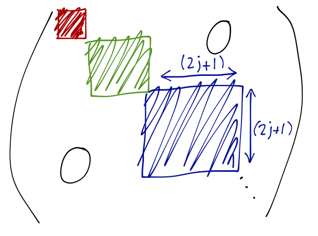
The \( (2j+1) \times (2j+1) \) blocks appearing in this matrix are the Wigner D-matrices for each \( j \); this shows explicitly the decomposition of our reducible rotation matrix (on the direct-product states) to a direct sum over irreducible representations (each one corresponding to a single Wigner D-matrix.)