Last time, we ended by gathering together our results for the fine structure of hydrogen, which come from the Hamiltonian
\[ \begin{aligned} \hat{H}_{fine} = \hat{H}_0 + \hat{W}_{rel} + \hat{W}_{SO} + \hat{W}_D. \end{aligned} \]
Specializing to the \( n=2 \) energy levels, we found the following results:
\[ \begin{aligned} \Delta E_{2s} = -\frac{5}{64}\alpha^2 \ \textrm{Ry}, \\ \Delta E_{2p,j=1/2} = -\frac{5}{64}\alpha^2 \ \textrm{Ry}, \\ \Delta E_{2p,j=3/2} = -\frac{1}{64} \alpha^2\ \textrm{Ry}. \end{aligned} \]
We noted that the unexpected "accidental" degeneracy between the \( 2s \) and \( 2p,j=1/2 \) energy levels is actually due to the fact that in the full relativistic solution, energy levels depend only on \( n \) and \( j \).
I should further note that despite our best efforts to be careful, we have not reproduced the experimental situation quite right; the \( 2s \) and \( 2p_{1/2} \) states are not degenerate in reality! There is one important effect which we have neglected, that we cannot deal with using our current framework, namely the quantum mechanical nature of the electromagnetic field itself. The missing effect gives rise to the Lamb shift, which is subleading to everything we've studied so far; it arises as an order \( \alpha^3 \) correction to the unperturbed energy level.
For these particular energy levels, the splitting corresponds to a frequency of \( 1060 \) MHz - to be compared to \( \sim 2000 \) THz from the difference between the \( n=2 \) and \( n=1 \) orbital energy levels, or \( 10 \) GHz for the fine splitting between \( 2p,j=1/2 \) and \( 2p,j=3/2 \) that we just found.
Hyperfine Hamiltonian
In all of the above, we have been focused completely on the electron and have essentially ignored the proton itself as anything but a static charge. Since the proton is so much heavier than the electron, this is mostly a reasonable approximation. However, the proton is in fact a spin-1/2 particle like the electron, so we should account for its spin degree of freedom as well; this will lead to new magnetic effects.
As you saw on the homework, the spin of the proton is conventionally denoted by \( \hat{\vec{I}} \). As with the electron, the proton's spin has an associated magnetic moment,
\[ \begin{aligned} \hat{\mu}_I = \frac{g_p \mu_n}{\hbar} \hat{\vec{I}}. \end{aligned} \]
\( \mu_n \) is the "nuclear magneton",
\[ \begin{aligned} \mu_n = \frac{e\hbar}{2m_p}, \end{aligned} \]
while \( g_p \) is the gyromagnetic ratio of the proton. For the electron, \( g_e \approx 2 \); the proton is a rather more complicated spin-1/2 object, and its g-factor is \( g_p \approx 5.6 \). Although the electron and proton carry the same angular momentum (eigenvalues \( \pm \hbar/2 \)), the tiny size of the nuclear magneton relative to the Bohr magneton appearing in the spin-orbit interaction means that any effects due to nuclear spin will be further suppressed by \( m_e / m_p \). These will all be \( \sim 2000 \) times smaller than the fine-structure terms, and are known as hyperfine corrections.
A careful study of the system leads to three terms once again at the hyperfine level: a spin-orbit coupling \( \hat{\mu}_I \cdot \hat{\vec{L}} \), a direct coupling between the nuclear and electron spins \( \sim \hat{\mu}_I \cdot \hat{\vec{S}} \), and a final spin-spin term containing a delta function, which is the hyperfine analogue of the Darwin term. I won't write the full hyperfine Hamiltonian out here, but you can find it in chapter 12 of Cohen-Tannoudji, among other places. We will make use of only the last one of the hyperfine terms:
\[ \begin{aligned} \hat{W}_{hf} \supset \frac{8\pi g_p e^2}{3 m_e m_p c^2} (\hat{\vec{S}} \cdot \hat{\vec{I}}) \delta(r). \end{aligned} \]
This term is known as the contact term; it's the only one that contributes to the 1s hyperfine splitting.
\( n=1 \) hydrogen: hyperfine structure
Now we'll briefly consider the hyperfine structure, this time moving back down to the \( n=1 \) energy level. The analysis is straightforward but much more complex for higher \( n \) states, and the hyperfine interactions will actually split the \( 1s \) state, unlike the fine-structure terms.
There is still a fine-structure correction to the \( 1s \) energy level, of course. You can verify easily that the values of the fine-structure terms are
\[ \begin{aligned} \ev{\hat{W}_{rel}} = -\frac{5}{8} \alpha^2\ \textrm{Ry}, \\ \ev{\hat{W}_D} = \frac{1}{2} \alpha^2\ \textrm{Ry}, \end{aligned} \]
and the spin-orbit term is again zero for an \( s \) orbital. Thus, the overall energy of the \( 1s \) level is shifted down by
\[ \begin{aligned} \Delta E_{1,f} = -\frac{1}{8} \alpha^2\ \textrm{Ry}. \end{aligned} \]
There is no splitting induced by this correction. Including the spin of the electron and now also of the proton, there are four degenerate states within the \( 1s \) level; we can write them in the basis
\[ \begin{aligned} \ket{s i; m_s m_i} \end{aligned} \]
suppressing the \( n \) and \( l \) labels which are constant here. Now, we consider the hyperfine interactions. As I noted before, two of the three interactions vanish for the \( 1s \) state; one is a spin-orbit type term which vanishes when \( l=0 \), and the other is a dipole-dipole interaction which vanishes due to the spherical symmetry of an \( s \) state. That just leaves us with the contact term. Plugging in the radial wavefunction \(|R_{10}(0)|^2\), it's easy to show that
\[ \begin{aligned} \ev{\hat{W}_{hf,C}} = \left(\frac{2}{3 \hbar^2} g_p \frac{m_e}{m_p} \left( 1 + \frac{m_e}{m_p}\right)^{-3} \alpha^2\ \textrm{Ry}\right) \ev{\hat{\vec{I}} \cdot \hat{\vec{S}}} \\ \equiv A \ev{\hat{\vec{I}} \cdot \hat{\vec{S}}}. \end{aligned} \]
Notice that the constant \( A \) is easily seen to be of order \( (m_e / m_p) \alpha^2 \), much smaller than the fine-structure terms. With a spin-spin interaction, and a set of degenerate states, we have to diagonalize by moving to a total spin basis,
\[ \begin{aligned} \hat{\vec{F}} = \hat{\vec{I}} + \hat{\vec{S}}. \end{aligned} \]
The new states will be labeled \( \ket{s i; f m_f} \). The addition of two spin-1/2 angular momenta is a problem we've solved before; the four states split into an \( f=1 \) triplet, and an \( f=0 \) singlet. As usual, we rewrite the spin dot product as
\[ \begin{aligned} \hat{\vec{I}} \cdot \hat{\vec{S}} = \frac{1}{2} (\hat{F}{}^2 - \hat{S}{}^2 - \hat{I}{}^2). \end{aligned} \]
The resulting energy eigenvalues are
\[ \begin{aligned} \ev{\hat{W}_{hf,C}}_{f=1} = \frac{A\hbar^2}{4} \\ \ev{\hat{W}_{hf,C}}_{f=0} = \frac{-3A\hbar^2}{4}. \end{aligned} \]
So the hyperfine interaction only partially removes the degeneracy; the three \( f=1 \) states remain degenerate.
Let's combine everything that we've found so far and sketch a complete diagram of the energy eigenvalues for the first two hydrogen orbital levels. (I will include the \( n=2 \) hyperfine corrections in my sketch, although we won't work them out explicitly here.) This diagram is just a sketch, and is certainly not to scale!
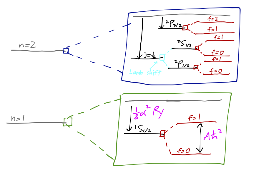
The value of the hyperfine splitting of \( 1s \) hydrogen is worth a closer look. If we calculate the energy difference between the \( f=1 \) and \( f=0 \) levels and convert to a light frequency by \( E = h \nu \), we find that
\[ \begin{aligned} \nu = \frac{A\hbar}{2\pi} = 1420.406...\ \textrm{MHz} \end{aligned} \]
or in terms of a wavelength, \( \lambda = 21 cm \). This radio-frequency light (also known as the "H-I spectral line") is extremely important to astrophysicists, because interstellar space is full of dust which can block substantial amounts of visible light, but which is mostly transparent to radio frequencies. This transition giving rise to the 21 cm light, incidentally, can be thought of as a rather simple ``spin-flip" transition in which the spins of the electron and proton go from parallel to anti-parallel. This fact was famously memorialized on the golden plaque attached to the Pioneer and Voyager space probes with the following diagram:
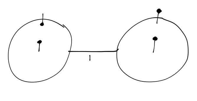
The other contents of the plaque use the 21cm line to provide units of time and length.
Invitation to quantum field theory
Trying to attack the relativistic corrections to the hydrogen spectrum one by one above is perfectly okay, but at some point it's better to just write down a treatment which is fully compatible with special relativity. As I said, the Dirac equation (which you'll probably see next semester) is an important first step towards doing just that: it describes the motion of the electron, or any other spin-1/2 particle, in a fully relativistic way. (There is a similar generalization for spin-zero particles, known as the Klein-Gordon equation.)
However, even the Dirac equation turns out to be a small part of the complete story, which is quantum field theory. The idea of quantum field theory most naturally arises as an answer to a completely different question, but we'll come back to relativity in a moment.
The key word there is "field". A field \( F \) is a physical object which takes on some value everywhere in space and time, i.e. \( F = F(\mathbf{x},t) \). This is as opposed to a particle, which (classically) has a definite position in space. You're familiar with the electromagnetic fields, of course, but another classical example is a string moving in one dimension, for which the displacement \( y(x,t) \) is a field.
Of course, we know that in quantum mechanics, our particles no longer have definite positions, but rather have wave-like properties of their own, described by the wavefunction \( \psi(x,t) \) which gives the probability density for that particle's location. Technically the wavefunction itself is a field, but don't get confused - it's still describing the physics of a single point-like particle.
The more appropriate question would be: how do we quantize something like the vibrating string which is already described by a field? Or, more urgently, how do we quantize the electromagnetic field? (We have dealt with such fields in quantum mechanics, but only as classical backgrounds; quantization of light requires quantum field theory.)
Borrowing a diagram from Sidney Coleman, we can think of two procedures, quantization and the continuum limit. Quantum field theory is what results from combining both procedures:
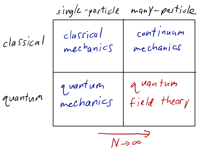
It should be pointed out that we don't have to use a continuous theory to study, say, a condensed matter system. Often, such systems aren't even continuous, but exist on a real and finite lattice: we can describe all of their physics in principle just using the Schrodinger equation. But this quickly becomes completely intractable for any realistic system, where there can be \( 10^{24} \) particles or more to work with. A continuous description is very powerful for understanding the collective properties of such a system, particularly in the context of phase transitions and critical phenomena.
What about the connection to high-energy physics? Our diagram above reminds us that there's another limit we already understand for classical systems, the relativistic limit - what is the appropriate extension of quantum mechanics there?
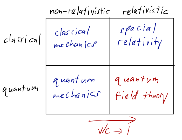
At the intersection of quantum mechanics and special relativity, we find quantum field theory again! This should come as a surprise - it's not obvious that this should be true. Why should we need continuous fields to understand the relativistic behavior of a single particle?
The simplest answer is that it is true: there were many attempts to simply promote single-particle descriptions such as the Schrodinger equation to relativistic equations, and they failed spectacularly, giving states with negative energy and violation of the laws of probability. But there are two other explanations which can give us a bit more physical insight. First, relativity implies matter-energy equivalence with the equation \( E=mc^2 \). Suppose we trap a particle and localize its position to within some uncertainty \( \Delta x \). The uncertainty principle tells us that \( \Delta p \Delta x\geq \hbar \), or
\[ \begin{aligned} \Delta E \Delta x \geq \hbar c. \end{aligned} \]
using \( E \approx pc \) for large enough momentum. If this uncertainty is sufficiently large, then there is potentially enough energy in the system to pop new particles out of the vacuum: in other words, we are now uncertain about even how many particles are in our trap. The threshold for this is \( \Delta E \gtrsim mc^2 \), or
\[ \begin{aligned} \Delta x = \lambda_C \sim \frac{\hbar}{mc}. \end{aligned} \]
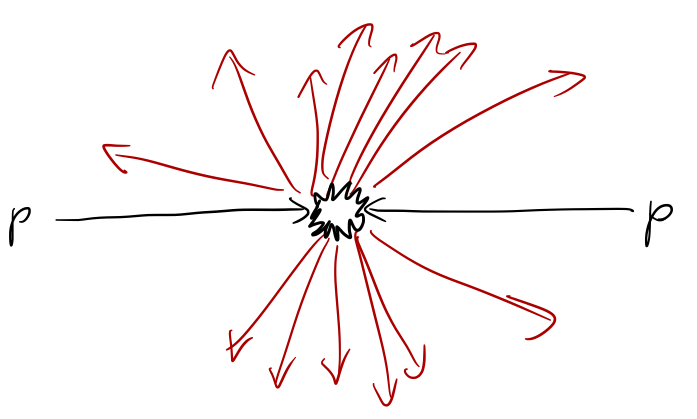
This length scale is known as the Compton wavelength of a particle, and we can think of it as the length scale at which a non-relativistic, single-particle description of the system has to break down. We can observe this experimentally: for example, at the Large Hadron Collider, collisions of two protons frequently produce many different final-state particles.
Strictly speaking, creation of particles from the vacuum can't happen completely arbitrarily. The electron, for example, is stable and can't be created from, or decay into, the vacuum state. On more general grounds, just creating a single electron out of nothing would violate charge conservation. But if there is an antiparticle with exactly opposite properties to the electron, then we can always create a particle-antiparticle pair from energy, and no symmetries are violated. (And indeed there is - the positron!)
The existence of antiparticles is an experimental fact, but it also gives us one more motivation for why quantum field theory is needed to combine relativity and quantum mechanics. Let's consider the probability amplitude for a quantum mechanical particle to propagate from the origin to another point \( \mathbf{x} \). We know from QM that we can write this as the matrix element of the time evolution operator between two position eigenstates:
\[ \begin{aligned} U(\mathbf{x},t) = \bra{\mathbf{x}} e^{-i\hat{H} t} \ket{\mathbf{x}=\mathbf{0}} \end{aligned} \]
Consider a completely free particle, so its Hamiltonian is just the kinetic energy \( \hat{H} = \hat{p}^2 / 2m \). We can evaluate by inserting a complete set of momentum states:
\[ \begin{aligned} U(\mathbf{x},t) = \int \frac{d^3 p}{(2\pi)^3} \bra{\mathbf{x}} e^{-i(\hat{p}^2/2m)t} \ket{\mathbf{p}} \sprod{\mathbf{p}}{\mathbf{x}=\mathbf{0}} \\ = \int \frac{d^3 p}{(2\pi)^3} e^{-i(\mathbf{p}^2/2m)t} e^{i\mathbf{p} \cdot \mathbf{x}}. \end{aligned} \]
This is a standard Gaussian integral, for which it's worth remembering the general result:
\[ \begin{aligned} \int d^n x\ e^{-\frac{1}{2} \mathbf{x}^T \cdot A \cdot \mathbf{x} + \mathbf{b}^T \cdot \mathbf{x}} = \sqrt{\frac{(2\pi)^n}{\det A}} e^{\frac{1}{2} \mathbf{b}^T\cdot A^{-1}\cdot \mathbf{b}} \end{aligned} \]
Our "matrix" \( A \) here is just the 3x3 identity times \( -it/m \), while \( \mathbf{b} \) is just \( i\mathbf{x} \), so combining we find
\[ \begin{aligned} U(\mathbf{x},t) = \left( \frac{m}{2\pi i t} \right)^{3/2} e^{im \mathbf{x}^2 / 2t}. \end{aligned} \]
This is all well and good, but you'll notice immediately that this expression is non-zero for any finite \( t \) and any \( \mathbf{x} \) - which implies that if we fix \( \mathbf{x} \) and pick a small enough \( t \), we will predict a non-zero probability for propagation faster than the speed of light. Thus, our amplitude leads to violation of causality!
You might expect that the culprit here is the use of the non-relativistic energy, and we could fix things by using \(E = \sqrt{\mathbf{p}^2 + m^2c^2}\) instead. By the same steps as above, this leads instead to the result
\[ \begin{aligned} U(\mathbf{x},t) = \int \frac{d^3p}{(2\pi)^3} e^{-ict \sqrt{\mathbf{p}^2 + m^2c^2}} e^{i\mathbf{p} \cdot x}. \end{aligned} \]
This is not a Gaussian integral, but we can do the angular part of the integral and the method of stationary phase to find that asymptotically, for \( x^2 \gg (ct)^2 \), we have
\[ \begin{aligned} U(\mathbf{x},t) \sim e^{-m|x|}. \end{aligned} \]
This is at least an improvement, because we have exponential suppression outside of the light cone instead of just oscillatory behavior; but it still implies propagation faster than light, which leads to violations of casuality in special relativity (and is inconsistent with experiment!)
In full quantum field theory, there are two parts to the resolution of this question. The first is that once we allow quantum fields, the propagator \( U(\mathbf{x},t) \) doesn't really mean the same thing anymore; the particles at both \( 0 \) and \( \mathbf{x} \) are both excitations of the same field, but they could be separate single-particle excitations - we can't really "track" the particle from initial to final point. We will have to define a modified version of the propagator to ask the more precise question: does the order of measurements matter between two spacelike-separated points?
And the answer will turn out to be no, but only because we will find two terms that individually are only exponentially suppressed, but that will cancel exactly. The two terms are exactly related to propagation of particles, and propagation of antiparticles - both are required. So in quantum field theory, the existence of antiparticles is required for compatibility with special relativity and causality!