Physics 3220, Fall '97. Steve Pollock.

Gas. Ch. 11 - Angular Momentum

3220 - Notes, lecture 39 (Mon, Nov 24, 1997)

Here is the previous lecture

Here is the Next lecture

Back to the list of lectures

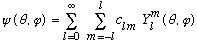
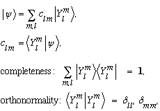
The Ylm's are a complete orthonormal set of functions, because they are eigenvectors of a pair of commuting Hermitian operators, L^2 and L_z.

(See our discussion/proof of this back in Ch. 6.)

This means that any function of theta and phi can be written

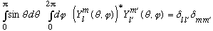
and orthonormality of the Ylm's, which would be written as:

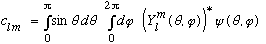
tells us what those c's are:

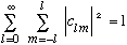
If the function is normalized, then as always, |c_lm|^2 tells the probability that the particle would give a measurement of L^2 giving , and L_z giving .

If we want the total probability of measuring l (irrespective of m), then

Prob(l)=

Completeness tells us .

In Dirac notation, we would write all the above ideas like this:

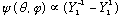
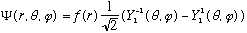
Example:

Suppose .

(unfortunately, this wave function is not normalizable, because of the bad behavior of f(r) at infinity, but never mind. It's so simple I'll go ahead and use it, and ignore overall normalization. We're really only interested in the angular part here anyway. Assume f(r) and are separately normalized.)

We can look at the angular part of this function (sin[theta] cos[phi]) and decompose it in terms of Ylm's. Let me remind you what the lowest Ylm's look like, and we can do it by inspection, rather than having to do a bunch of integrals:

If you mess around a bit, you quickly notice that

,

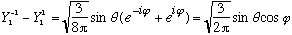so . Now I can normalized the angular part by inspection, since I know the Ylm's are themselves all normal:

Some probabilities, which I get by inspection (squaring coefficients):

Prob(l=0)=0, Prob(l=1)=1, Prob(any other l)=0,

Prob(m=1)= 50%, Prob(m=0)=0, Prob(m=-1)=50%, Prob(any other m)=0.

As one final example here, Gas considers the case V=0. Note that in x,y,z space the solution

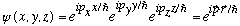
is immediately a solution to the Schrod Eq. (It's just a plane wave in 3-D).

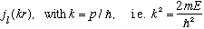
But let's look in spherical coordinates: We've already (sort of) looked at this in r space, in Ch. 10, and found

R(r)=

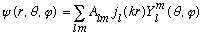
Thus, our full solution must be of the form

Let's choose the z direction as the same as p. Our x,y,z solution is

.

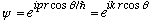This must be equal to our alternative form, i.e.

By inspection, there is no phi dependence on the lhs: only m=0 can contribute. The Y_l0 functions have the form

,

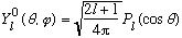where P_l is just a plain old Legendre Polynomial, which you can look up in Boas.

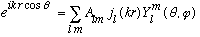
Now we can use our angular expansion:

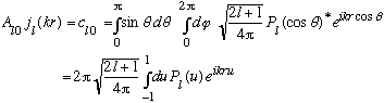
Gas uses some tricks to evaluate this integral: (he looks at what happens for small p, but then argues that the A_l0's are constants, independent of p!) giving:

.

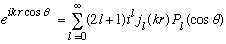A useful and important formula, which you may have encountered in E+M as well (?). This formalism will get used when we discuss collisions in 3-D (next semester), but has taken us a bit afield for the moment.

In this short chapter we have derived essentially all the basic properties of the Ylm's by using operator methods, with raising and lowering operators. We now return to the problem of the radial equation, this time for the hydrogen atom potential.

Gas. Ch. 12 - The Hydrogen Atom

We are all set up to discuss the potential V(r) = -Z e^2/r, the hydrogenic electric potential. (This describes not just hydrogen, but Li+, Be++, etc.) If we use reduced mass we will also be easily able to describe the differences between hydrogen, deuterium, and tritium.) We have come full circle - we began the semester with Bohr's attempt to form a "quantum picture" of hydrogen. Armed with his crude ideas, following the lead of De Broglie, and then Heisenberg, and Schrodinger, we are now equipped with a full fledged mathematical framework. Bohr only had a few postulates, and no consistent framework within which to compute anything but the simplest observable (energy). He got that right, but just about everything else (radii, angular momentum) was not right. We know how to compute the wave function now, which tells us everything there is to know about an electron in hydrogen - not just its energy, but its momentum, angular momentum, parity, position, potential and kinetic energy separately, etc.

We've already solved the angular part of the 3-D Schrod Eqn. The Ylm's are universal functions, valid for any central potential. In a certain sense 2/3 of our work is done! We only need to study the radial equation. As always, let me define a new function u(r)=r R(r), which we thus require goes to zero at r=0. The radial equation for u, as described in Ch. 10, is

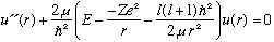
I usually define some variable = -2mE/hbar^2, but this time (for reasons which will be clear soon), I'm going to define

(which is manifestly positive for bound states.)

Our radial equation looks like

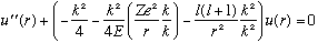
where I introduced a couple of gratuitous "1"'s = "k/k"'s for later use...

Now, as usual, I like to switch to unitless variables. Here, the natural "unitless radius" variable is just kr, so we define

.

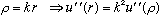Also I'll define another unitless constant for you (it's a bit inobvious!)

.

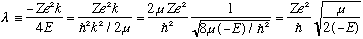None of those expressions is "obviously" unitless to me, but one more manipulation does make it clear, if you remember :

.

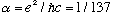Lambda is dependent only on the energy. If we can solve for it, we immediately learn the energy.

Our radial equation has turned into

,

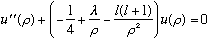a unitless, second order ODE. Here is the Next lecture