Physics 3220, Fall '97. Steve Pollock.

3220 - Notes, lecture 29 (Fri Oct 31 1997)

Here is the previous lecture

Here is the Next lecture

Back to the list of lectures

From now on, all the rest of the solutions can be normalized using operator tricks! Gas. has a method which I do not find very intuitive. So, here's an alternative. Suppose we do have a normalized . (We already know its energy, E_n = (n+1/2) .)

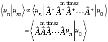
Now, let's find the next higher wave function, . I already know that it must be proportional to . We just need to find the proportionality constant. Let's just figure out the norm of (it won't in general be 1)

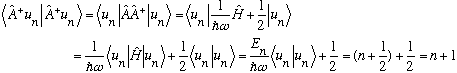
From which I conclude that

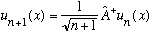
Is properly normalized!

To summarize,

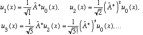
(I hope the generalization to the n'th state is obvious)

Example:

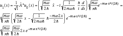
You derived this wave function on HW 8, using Hermite polynomials and normalizing by hand. Here, all you had to do was take one derivative, and that's it. In principle, it's purely mechanical to generate any wavefunction u_n(x) now, with proper normalization. You don't have to look up any Hermite stuff, and you don't have to do any integrals. (Indeed, you are generating the Hermite polynomials.)

Comment: I have shown that I've found an infinite number of solutions this way. But how do I know that I haven't missed any? Couldn't there be two different "ladders" of solutions, displaced by some small amount, and I missed the second one entirely? The answer is no! If there were another ladder, it would also have to have a lowest rung, and thus a lowest energy eigenfunction, call it v_0. This state would still have to satisfy Av_0(x)=0. But, remember, this was a first order ordinary differential equation. These only have one unique solution! So, u_0 and v_0 must be one and the same; we have really found all possible solutions.

In Ch. 6, we proved quite generally that eigenvectors with distinct eigenvalues are orthogonal, thus we also have

I can prove this to you more directly, too, if you like:

Proof:

Suppose m>n. Then,

But m>n. The first n of those A's operating on u_n brings it down to u_0. (With some proportionality constant we don't care about). But m>n, so we still have some A's sitting there. The very first one kills u_0, and we get 0! (The argument if m<n is similar.)

(When m=n, the u_n's are by definition normalized. I showed it on p. 7-6)

As we discussed in Ch. 6, we can expand any state vector (whatsoever) . Orthonormality means that .

Remember, |c_n|^2 tells you the probability of measuring the energy E_n.

We have completely solved the Harmonic Oscillator using operator methods, recovering all the results we had gotten from the power series method, with far less algebraic grief. These operator techniques are also rather tricky (and inobvious, the first time around!) but they are useful in other problems as well. We will see a very similar game later this semester when we deal with angular momentum in 3-D, and again in Quantum II when we deal with electromagnetic radiation (photons have a lot in common with Harmonic Oscillators). The technique really comes into its own when one studies relativistic quantum field theory, where these operator methods are the main game in town....

To finish up this chapter, we will study a couple more useful features of Dirac notation, while we look at the Time dependence of wave functions.

Recall that one of the postulates of Q.M. is the time dependent S.E:

I claim that

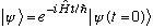satisfies the above equation.

This is a (rather formal) way of writing down the time dependence of any wave function. Notice that it is not just "multiply by some phase", because there's an H operator up there in the exponential! (It's only the simple (usual) phase you might expect if is a pure eigenfunction of energy, i.e. if H psi = E psi.)

Proof: Just plug in my claim, and see that it satisfies the S.E.:

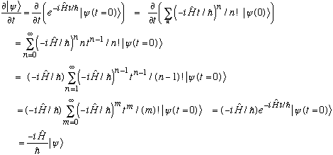
I.e. the solution that I wrote down does indeed satisfy the time dependent S.E., which is after all what I wanted to show.

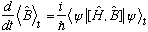
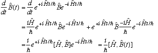
Now consider any operator B which has no explicit time dependence, and lets look at <B>(t):

What this means is that I could, if I wanted to, define a time dependent operator related to the original one in the following way:

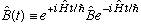
What I just showed is

It's purely a matter of definitions, notation, and ultimately of convenience which I choose. I can think of the time dependence as "belonging to the wave functions", or else as "belonging to the operator". With our new attitude in the last chapter of "the operator is the key player", it's nice to see that even time dependence can be attributed to the operators (rather than the states).

This operator-centric worldview is sometimes called the Heisenberg picture.

Your state vector is fixed and constant in time. All the time dependence of the problem is shifted to operators. The wave function doesn't have all that much importance in this way of thinking of things.

On the other hand, the wave-fn-centric worldview <-> Schrodinger picture.

Here, the state vector explicitly depends on time, the operators are fixed constant things for all time.

In the last chapter, remember we derived an expression something like this:

(for time independent operators).

What do we have from our results above?

It looks very similar to what I had before, except there's no expectation value involved. If you sandwich the wave function at t=0 around both sides, you will reproduce our old result. But, this new equation is an operator expression. There is no matrix element involved, the states are irrelevant. We have found how operators evolve in time no matter what states you're interested in.

This is quite a powerful tool - it teaches you about how just about any physical observable (i.e. any operator) changes with time.

Example:

Let's first look at H itself (assuming no explicit time dependence, of course.)

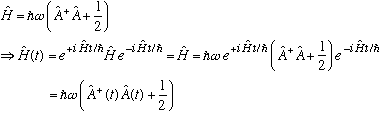
So we know what the "time dependence" of the Hamiltonian is (none!), and how it relates to the time dependence of A, which we'll get to soon.

It might be interesting to see what the time dependence of some commutators are, e.g.:

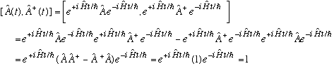
This commutator is time independent. We can make use of this in a (similar) derivation of the commutator of H and A. I leave it to you to check that, starting from our old identity you can fairly easily show

.

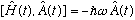From this, we know the time dependence of A:

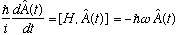
This is a first order differential equation, which we'll solve below. But first, note the similar relation for A(dagger):

.

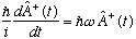
Let's go ahead and solve these little differential equations:

and similarly,

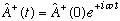
This is the time dependence of A and A(dagger), which we noted above.

We can make use of these in other ways, e.g., they provide a lovely shortcut to finding the time dependence of other operators, like x and p, just by writing down the original definitions of A and A(dagger)

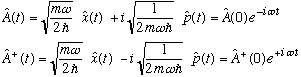
You can view the above as two equations in the two unknowns x(t) and p(t), and in this way we will know how those operators evolve in time:

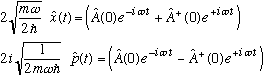
At time t=0, we can solve the equation at the top of the page for A and A(dagger) in terms of x(0) and p(0), and plug in here, giving (check this)

This last result is simple, and very powerful. Suppose you give me a state, any state (doesn't have to be an eigenfunction of energy) at time t=0. I just sandwich the above (simple!) expression for x(t) with that state at t=0, and I have found <x>(t), the time dependence of the position.

(And, of course, you can easily do the same for momentum)

It is as I promised way back in the beginning. The time dependence in quantum mechanics is really pretty simple, all the hard work goes into finding out what the state is at t=0 (i.e., solving Schrodinger's time independent equation) and then the Hamiltonian (or in this case, commutators with the Hamiltonian) tells you about time evolution in a very simple way. (I have, however, implicitly assumed that H has no explicit time dependence; this whole discussion has been only about operators with no explicit time dependence, that's the only caveat...)

Here is the Next lecture